11. Planning under $v^*$ realizability (TensorPlan I.)

PDF Version

In the last lecture we saw that under $q^*$ linear realizability, query-efficient fixed-horizon online planning with a constant suboptimality gap is intractable provided that there is no limit on the number of actions. In particular, the MDPs that were used to show intractability use $e^{\Theta(d)}$ actions, where $d$ is the dimension of the feature-map that realizes the optimal action-value function. At the end of the lecture, we also noted that intractabality also holds for undiscounted infinite horizon problems under $v^*$ linear realizability in the regime when the number of actions scales linearly with $d$. In this lecture we further dissect $v^*$ realizability, but return to the fixed horizon setting and we will consider the case when the number of actions is fixed. As it turns out, in this case, query-efficient online planning is possible.

Before giving the details of this result, we need to firm up some and refine other definitions. First, $v^*$ realizability under a feature map $\phi=(\phi_h)_{0\le h \le H-1}$ in the $H$-horizon setting means that

\[\begin{align} \inf_{\theta\in \mathbb{R}^d} \max_{0\le h \le H-1}\|\Phi_h \theta - v^*_{h} \|_\infty = 0\,, \label{eq:vsrealizability} \end{align}\]

where $v^*_h$ is the optimal-value function when $H-h$ steps are left (in particular, $v^*_H=\boldsymbol{0}$). Again, this uses the indexing introduced in the previous lecture. In what follows, without the loss of generality we assume that the feature map is such that all the feature-vectors lie within the a ($2$-norm) ball of radius one. When realizability holds with a parameter vector bounded in $2$-norm by $B$, we say that $v^*$ is $B$-realizable under the feature map $\phi$.

We also slightly modify the interaction protocol between the planner and the simulator, as shown on the figure below. The main new features are introducing stages, and restricting the planners to access states and features only through local calls to the simulator.

drawing
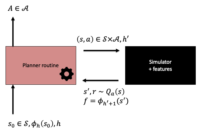
Illustration of the interaction protocol between the planner and the simulator.

Because in fixed-horizon problems the stage index influences what actions should be taken, the planner is called with an initial state $s_0$ and a stage index $h$. For defining the policy induced the planner, it is assumed that the planner is first called with $h=0$ at some state, then it is called with $h=1$ with a state obtained following a transition by taking the action returned by the planner, etc. While interacting with the simulator, the planner is restricted to use only states that it has encountered before. Also, the planner can feed a stage index to the simulator, to get the features of the next state corresponding to the incremented input stage index. There is no other access to the features. Note also that just like in the previous lecture, we allow the MDPs to generate random rewards.

In this setting a $\delta$-sound planner is one which, under the above protocol, induces a policy of the MDP whose simulator it interacts with which is at most $\delta$-suboptimal.

Theorem (query-efficient planning under $v^*$-realizability): For any integers $A,H>0$ and reals $B,\delta>0$, there exists an online planner $\mathcal{P}$ with the following properties:

The planner $\mathcal{P}$ is $\delta$-sound for the $H$-horizon planning problem and the class of MDP-feature-map pairs $(M,\phi)$ such that $v^*$ is $B$-realizable under $\phi$ and $M$ has at most $A$ actions and its rewards are bounded in $[0,1]$;
The number of queries used by the planner in each of its call is at most

\[\begin{align*} \text{poly}\left( \left(\frac{dH}{\delta}\right)^A, B \right) \end{align*}\]

Note that for $A>0$ fixed the query-cost is polynomial in $d,H,1/\delta$ and $B$. It remains to be seen whether this bound can be improved. However, this is somewhat of a theoretical question as under $v^*$-realizability, even if the coefficients $\theta\in \mathbb{R}^d$ that realize $v^*$ are known, in the lack of extra information, one needs to perform $\Theta(A)$ simulation calls to be able to get good approximations to the action-value function $q^*$, which seems necessary for inducing a good policy. Hence, the query cost must scale at least linearly with $A$, hence, no algorithm is expected to be even query-efficient when the number of actions is large.

TensorPlan: An optimistic planner

The planner that is referred to in the previous theorem is called TensorPlan. The reason for this name will become clear after we describe the algorithm.

TensorPlan belongs to the class of optimistic algorithms. Since knowing $\theta^*$, the parameter vector that realizes $v^*$, would be sufficient for acting near-optimally, the algorithm aims to find a good approximation to this vector.

A suitable estimate is constructed in a two-step process:

The algorithm maintains a non-empty “hypothesis” set $\Theta\subset \mathbb{R}^d$, which contains those parameter vectors that are consistent with the data that the algorithm has seen. The details of the construction of this set are at the heart of the algorithm and will come soon.
Given $\Theta$, an estimate $\theta^+$ is produced by solving a maximization problem:

\[\begin{align} \theta^+=\arg\max_{\theta\in \Theta} \phi_0(s_0)^\top \theta\,. \label{eq:optplanning} \end{align}\]

Here, $s_0$ is the initial state of the episode, i.e., this is the state the planner is called when $h=0$. Recalling that $\phi_0(s_0)^\top \theta^* = v_0^*(s_0)$, we see that provided that $\theta^*\in \Theta$,

\[v_0(s_0;\theta^+)\ge v_0^*(s_0)\,,\]

where, for convenience, we introduce $v_h(s;\theta) = \phi_h(s)^\top \theta$. When $\theta^+$ is close enough to $\theta^*$, one hopes that the policy induced by $\theta^+$ will be near-optimal. Hence, the approach is to “roll out” with the induced policy (using the simulator) and verify whether during the rollout the data received is consistent with the Bellman equation, and as a result of this, also whether the episode return observed is close to $v_0(s_0;\theta^+)$. When a contradiction to any of these is detected, the data can be used to shrink the set $\Theta$ of consistent parameter vectors.

The approach described leaves open the question of what we mean by a policy “induced” by $\theta^+$. The naive approach is to base this on the Bellman optimality equation, which states that

\[\begin{align} v_h^*(s) = \max_a r_a(s)+ \langle P_a(s), v_{h+1}^* \rangle \label{eq:fhboe} \end{align}\]

holds for $h=0,1,\dots,H-1$ with $v_H^* = \boldsymbol{0}$. If $\theta^+= \theta^*$, $v_h(\cdot;\theta^+)$ will also satisfy this equation and thus one might define the policy induced by $\theta^+$ that achieves the maximum above when $v_{h+1}^*$ is replaced by $v_{h+1}(\cdot;\theta^+)$. Consistency of $\theta^+$ would also mean checking whether \eqref{eq:fhboe} holds (approximately) when $v^*_{\cdot}(\cdot)$ is replaced in this equation by $v_{\cdot}(\cdot;\theta^+)$, which, one may imagine can be checked by generating data from the simulator.

While this may approach work, it is not easy to see whether it does. (It is open problem whether this works!) TensorPlan defines induced policies and consistency slightly differently. The changed definition allows not only for proving that TensorPlan is query-efficient, but it even makes the guarantees for TensorPlan stronger than what was announced above in the theorem.

What makes the analysis of the algorithm that is based on the Bellmean optimality equation difficult is the presence of the maximum in this equation. Hence, TensorPlan removes this maximum. Accordingly, the policy induced by $\theta^+$ is defined as any policy $\pi_{\theta^+}$ which in state $s$ and stage $h$ chooses any action $a\in \mathcal{A}$ which ensures that

\[\begin{align} v_h(s;\theta^+) = r_a(s)+ \langle P_a(s), v_{h+1}(\cdot;\theta^+) \rangle\,. \label{eq:tpcons} \end{align}\]

If there is no such action, $\pi_{\theta}$ is free to choose any action. We say that local consistency holds at $(s,h,\theta^+)$ when there exists an action $a\in \mathcal{A}$ such that \eqref{eq:tpcons} holds.

If there are multiple actions that satisfy \eqref{eq:tpcons}, any of them will do: Choosing the maximizing action is not enforced. However, when $v^*$ is realizable and $\theta^+=\theta^*$, any action that satisfies \eqref{eq:tpcons} will be a maximizing action and the policy induced will be optimal.

The advantage of the relaxed notion of induced policy is that with this choice, TensorPlan will also be able to compete with any deterministic policy whose value-function is realizable. This expands the scope of TensorPlan: Perhaps the optimal value function is not realizable with the features handed to TensorPlan, but if there is any deterministic policy whose value-function is realizable with them, then TensorPlan will be guaranteed to produce almost as much as reward as that policy. In fact, it will produce nearly as much reward as the policy that achieves the best value.

TensorPlan

To summarize, after generating a hypothesis $\theta^+$, TensorPlan will run a number of rollouts using the simulator so that for each state $s$ encountered TensorPlan first finds an action $a$ satisfying \eqref{eq:tpcons}. If this succeeds, the rollout continues by TensorPlan getting a next state from the simulator at $(s,a,h)$ and $h$ is incremented. This continues up to $h=H$, which ends a rollout. TensorPlan will run $m$ rollouts of this type and if all of them succeeds, TensorPlan stops and will use the parameter vector $\theta^+$ in the rest of the episode and the same policy $\pi_{\theta^+}$ as used during the rollouts. If during the rollouts an inconsistency is detected, TensorPlan will decrease the hypothesis set $\Theta$ and continue with a next experiment.

It remains to be seen why TensorPlan (1) stops with a bounded number of queries and (2) why it is sound.

Boundedness

We start with boundedness. This is where the change of how policies are induced by parameters is used in a critical manner. Introduce the discriminants:

\[\begin{align*} \Delta(s,a,h,\theta) = r_a(s) = \langle P_a(s)\phi_{h+1},\theta \rangle - \phi_h(s)^\top \theta\,. \end{align*}\]

Note that $\Delta(s,a,h,\theta)$ is just the difference between the right-hand and the left-hand side of \eqref{eq:tpcons}, where we plugged in the definition $v_h$ and $v_{h+1}$ and we define

\[P_a(s)\phi_{h+1} = \sum_{s'\in \mathcal{S}} P_a(s,s') \phi_{h+1}(s')\,;\]

thus $P_a(s)\phi_{h+1}$ is the “expected next feature vector” given $(s,a)$. Then, by definition, local consistency holds for $(s,h,\theta)$ if and only if there exists some action $a\in \mathcal{A}$ such that $\Delta(s,a,h,\theta)=0$. Exploiting that the product of numbers is zero if and only if some of them is zero, we see that local consistency is equivalent to

\[\begin{align} \prod_{a\in \mathcal{A}} \Delta(s,a,h,\theta) = 0\,. \label{eq:diprod} \end{align}\]

The reason this purely algebraic reformulation of local consistency is helpful is because the product of the discriminants can be see as a linear function of the $A$-fold tensor product of $(1,\theta^\top)^\top$.

To see why this holds, it will be useful to introduce some extra notation: For a real $r$ and a finite-dimensional vector $u$, we will denote by $\overline{ r u}$ the vector $(r,u^\top)^\top$ (i.e., adding $r$ to the first position and shifting down all other entries in $u$). With this notation, we can write the discriminants as an inner product:

\[\begin{align*} \Delta(s,a,h,\theta) = \langle \overline{r_a(s)\, (P_a(s)\phi_{h+1}-\phi_h(s))}, \overline{1 \, \theta} \rangle \end{align*}\]

Now, recall that the tensor product $\otimes$ of vectors satisfies the following property:

\[\begin{align*} \prod_a \langle x_a, y_a \rangle = \langle \otimes_a x_a, \otimes_a y_a \rangle\,, \end{align*}\]

where the inner product between two tensors is defined in the usual way, by overlaying them and then taking the sum of the products of the entries that are on the top of each other.

Based on this identity, we see that \eqref{eq:diprod}, and thus local consistency, is equivalent to

\[\begin{align*} \langle \underbrace{\otimes_a \overline{r_a(s)\, (P_a(s)\phi_{h+1}-\phi_h(s))}}_{D(s,h)}, \underbrace{\otimes_a \overline{1 \, \theta}}_{F(\theta)} \rangle = 0\,. \end{align*}\]

Note that while $F(\theta)\in \mathbb{R}^{(d+1)^A}$ is a nonlinear function of $\theta$, the above equation is linear in $F(\theta)$.

Imagine for a moment that the data $D(s,h)$ above can be obtained with no errors and assume that $v^*$ is realizable. Let $k = (d+1)^A$. We can think of both $D(s,h)$ and $F(\theta)$ taking values in $\mathbb{R}^k$ (this corresponds to “flattening” these tensors).

TensorPlan can be seen as an algorithm that generates a sequence $(\theta_1,x_1), (\theta_2,x_2), \dots$ such that $\theta_i\in \mathbb{R}^d$ is the $i$th hypothesis that TensorPlan chooses, $x_i\in \mathbb{R}^k$ is the $i$th data of the form $D(s,h)$ with some $(s,h)$ where TensorPlan detects an inconsistency. When inconsistency is detected, the hypothesis set is shrunk:

\[\Theta_{i+1} = \Theta_i \cap \{ \theta\,:\, F(\theta)^\top x_i=0 \},\]

and $\theta_{i+1}$ is chosen in $\Theta_{i+1}$ by \eqref{eq:optplanning}. Together with $\Theta_1 = B_2^d(B)$ (the $\ell^2$ ball of radius $B$ in $\mathbb{R}^d$), we have that for $i>1$,

\[\Theta_i = \{ \theta\in B_2^d(B)\,:\, F(\theta)^\top x_1 = 0, \dots, F(\theta)^\top x_{i-1}=0 \}.\]

Let $f_i = F(\theta_i)$. By its construction, for any $i\ge 1$, $\theta_i\in \Theta_i$ and hence $f_i$ is orthogonal to $x_1,\dots,x_{i-1}$. Also by its construction, $x_i$ is not orthogonal to $f_i$. Because of this, $x_i$ cannot lie in the span of $x_1,\dots,x_{i-1}$ (if it did, it would be orthogonal to $f_i$). Hence, the vectors $x_1,x_2,\dots$ are linearly independent. As there are at most $k$ linearly independent vectors in $\mathbb{R}^k$, Tensorplan will generate at most $k$ of these data vectors (in fact, for TensorPlan, this is $k-1$, can you explain why?). This means that after at most $k$ “contradictions” to local consistency, TensorPlan will cease to detect more inconsistencies and thus it will stop.

Soundness

It remains to be seen that TensorPlan is sound. Let $\theta^+$ be the parameter vector that TensorPlan generated when it stops. This means that during the $m$ rollouts, TensorPlan did not detect any inconsistencies.

Take a trajectory $S_0^{(i)},A_0^{(i)},\dots,S_{H-1}^{(i)},A_{H-1}^{(i)},S_H^{(i)}$ generated during the $i$th rollout of $m$ rollouts. Since there is no inconsistency along it, for any $0\le t \le H-1$ we have

\[\begin{align} r_{A_t^{(i)}}(S_t^{(i)}) = v_t(S_t^{(i)};\theta^+)-\langle P_{A_t^{(i)}}(S_t^{(i)}), v_{t+1}(\cdot;\theta^+) \rangle\,. \label{eq:constr} \end{align}\]

Hence, with probability $1-\zeta$,

\[\begin{align*} v_0^{\pi_{\theta^+}}(s_0) & \ge \frac1m \sum_{i=1}^m\sum_{t=0}^{t-1} r_{A_t^{(i)}}(S_t^{(i)}) - H \sqrt{ \frac{\log(1/\zeta)}{2m}} \\ & = \frac1m \sum_{i=1}^m\sum_{t=0}^{t-1} v_t(S_t^{(i)};\theta^+)-\langle P_{A_t^{(i)}}(S_t^{(i)}), v_{t+1}(\cdot;\theta^+)\rangle - H \sqrt{ \frac{\log(2/\zeta)}{2m}} \\ & \ge \frac1m \sum_{i=1}^m\sum_{t=0}^{t-1} v_t(S_t^{(i)};\theta^+)- v_{t+1}(S_{t+1}^{(i)};\theta^+) - (H+2B) \sqrt{ \frac{\log(2/\zeta)}{2m}} \\ & = v_0(s_0;\theta^+) - (H+2B) \sqrt{ \frac{\log(2/\zeta)}{2m}}\,, \end{align*}\]

where the first inequality is by Hoeffding’s inequality and uses that rewards are bounded in $[0,1]$, the equality after it uses \eqref{eq:constr}, the second inequality is again by Hoeffding’s inequality and uses that

\[\begin{align*} \langle P_{A_t^{(i)}} (S_t^{(i)}), v_{t+1}(\cdot;\theta^+)\rangle = \mathbb{E} [ v_{t+1}(S_{t+1}^{(i)};\theta^+) | S_t^{(i)},A_t^{(i)}] \end{align*}\]

and that $v_t$ is bounded between $[-B,B]$ (note that we could truncate $v_t$ to $[0,H]$ to replace $H+2B$ above by $2H$), while the last equality uses that $v_H(\cdot;\theta^+)=\boldsymbol{0}$ by definition and that $S_0^{(i)}=s_0$ by definition. Setting $m$ high enough ($m=\tilde O((H+B)^2/\delta^2)$) we can guarantee

\[v_0^{\pi_{\theta^+}}(s_0) \ge v_0(s_0;\theta^+)-\delta.\]

We now argue that this implies soundness.

Letting $\Theta^\circ \subset B_2^d(B)$ be the set of $B$-bounded parameter vectors $\theta$ such that for some deterministic policy $\pi$, $v^\pi = \Phi \theta$. By the definition of $D$ and $F$, for any $i\ge 1$, $\Theta^\circ \subset \Theta_{i}$ (no correct hypothesis is ever eliminated). It also follows that at any stage of the process,

\[v_0(s_0;\theta^+)\ge \max_{\theta\in \Theta^\circ} v^{\pi_{\theta}}_0(s_0).\]

Hence, when TensorPlan stops with parameter $\theta^+$, with high probability,

\[v^{\pi_{\theta^+}}_0(s_0)\ge v_0(s_0;\theta^+)-\delta \ge \max_{\theta\in \Theta^\circ} v^{\pi_{\theta}}_0(s_0)-\delta\,.\]

In particular, if $v^*$ is $B$-realizable, $v^{\pi_{\theta^+}}_0(s_0) \ge v^*_0(s_0)-\delta$. Thus, after stopping, for the rest of the episode, TensorPlan can safely use the policy induced by $\theta^+$.

Summary

So far we have seen that if somehow TensorPlan would be able to get $\Delta(s,a,h,\theta)$ with no errors, (1) it would stop after refining its hypothesis set at most $k$ times and (2) when it stops, with high probability it would return with a parameter vector that induces a policy with high value. Regarding the number of queries used, if obtaining $\Delta(s,a,h,\theta)$ is counted as a single query, TensorPlan would need at most $maH k =maH (d+1)^A$ queries ($m$ rollouts, for each of the $H$ states in the rollout, $A$ queries are needed).

It remains to be seen how to adjust this argument to the case when $\Delta(s,a,h,\theta)$ need to be estimated based on interactions with a stochastic simulator.

Notes

It is not known whether TensorPlan can be computationally efficiently implemented. I suspect it cannot. This is because $\Theta_i$ is specified with a number of highly nonlinear constraints (in the parameter vector).
The essence of the construction here is lifting the problem into a higher-dimensional linear space. This is a standard technique in machine learning but in a very different context when data is mapped to a higher dimensional space to strengthen the power of linear predictors. The once popular RKHS methods take this to the extreme. Note that here, in contrast to this classic lifting procedure, the parameter vector is mapped through a nonlinear function to a higher dimensional space and the purpose is to simply have a clear grasp on why learning stops.
We call $\Delta$ here the discriminant function because what is important about it is that it discriminates between “good” and “bad” cases and it does it by using the special value of zero. Readers familiar with the RL literature will note, however, that $\Delta$ is nothing but, what is known as the “temporal difference error” (under some fixed action).
It is curious that the algorithm builds up a data-bank of critical data that it uses to restrain the set of parameter vectors and that it is quite selective in adding new data here. That is, TensorPlan may generate a lot more data then goes on the list $x_1,x_2,\dots$. If we wanted to be philosophical and would not mind antropomorphising algorithms, we could say that TensorPlan remembers what it is “surprised by”. This is very much unlike other algorithms, like LSVI-$G$, which may generate a lot of redundant data. The other difference is that TensorPlan uses the data to generate a hypothesis set. The choice of the parameter vector from this set is dictated by the optimization (reward maximization) problem solved by TensorPlan.
There are quite a few examples of optimistic algorithms in planning; there is a considerable literature of using optimisim in tree search. However, classics, such as the $A^*$ algorithm can also be seen as an optimistic algorithm (at least when used with an “admissible heuristic”, which is just a way of saying that $A^*$ uses an optimistic estimate of the values). The $LAO^*$ algorithm is another example. However, the real “homeland” of optimistic algorithms in online learning, a topic that will be covered later in the course.

Bibliographical notes

This lecture is entirely based on the paper

Weisz, Gellert, Philip Amortila, Barnabás Janzer, Yasin Abbasi-Yadkori, Nan Jiang, and Csaba Szepesvári. 2021. “On Query-Efficient Planning in MDPs under Linear Realizability of the Optimal State-Value Function.”

available on arXiv.