14. Politex
The following lemma can be extracted from the calculations found at the
end of the last lecture:
Lemma (Mixture policy suboptimality): Fix an MDP $M$. For any sequence \(\pi_0,\dots,\pi_{k-1}\) of policies, any sequence $\hat q_0,\dots,\hat q_{k-1}: \mathcal{S}\times \mathcal{A} \to \mathbb{R}$ of functions, and any policy \(\pi^*\), the mixture policy $\bar \pi_k = 1/k(\pi_0+\dots+\pi_{k-1})$ satisfies
\[\begin{align} v^{\pi^*} - v^{\bar \pi_k} & \le \frac1k (I-\gamma P_{\pi^*})^{-1} \underbrace{ \sum_{j=0}^{k-1} M_{\pi^*} \hat q_j - M_{\pi_j} \hat q_j}_{T_1} + \frac{2 \max_{0\le j \le k-1}\| q^{\pi_j}-\hat q_j\|_\infty }{1-\gamma} \,. \label{eq:polsubgapgen} \end{align}\]In particular, the only restriction is on policy $\pi^*$ so far and that is that it has to be a memoryless policy. To control the suboptimality of the mixture policy, one just needs to control the action-value approximation errors \(\| q^{\pi_j}-\hat q_j\|_\infty\) and the term $T_1$ and for this we are free to choose the policies \(\pi_0,\dots,\pi_{k-1}\) in any way we want them to be chosen. To help with this choice, let us now inspect \(T_1(s)\) for a fixed state $s$:
\[\begin{align} T_1(s) = \sum_{j=0}^{k-1} \langle \pi^*(s,\cdot),\hat q_j(s,\cdot)\rangle - \langle \pi_j(s,\cdot),\hat q_j(s,\cdot)\rangle \,, \label{eq:t1s} \end{align}\]where, abusing notation, we use \(\pi(s,a)\) for \(\pi(a|s)\). Now, recall that \(\hat q_j\) will be computed based on \(\pi_j\) while \(\pi^*\) is unknown. One must thus wonder whether it is possible to control this term?
Online linear optimization
As it happens, the problem of controlling terms of this type is the central problem studied in a subfield of learning theory, online learning. In particular, in online linear optimization, the following problem is studied:
An adversary and a learner are playing a zero-sum minimax game in $k$ discrete rounds, taking actions in an alternating manner. In round $j$ ($0\le j \le k-1$), first, the learner needs to choose a vector \(x_j\in \mathcal{X}\subset \mathbb{R}^d\). Then, the adversary chooses a vector, \(y_j \in \mathcal{Y}\subset \mathbb{R}^d\). Before its choice, the adversary learns about all previous choices of the learner, and the learner also learns about all previous choices of the adversary. They also remember their own choices. For simplicity, let us constraint the adversary and the learner to be deterministic. The payoff to the adversary at the end of the $k$ rounds is
\[\begin{align} R_k = \max_{x\in \mathcal{X}}\sum_{j=0}^{k-1} \langle x, y_j \rangle - \langle x_j,y_j \rangle\,. \label{eq:regretdefolo} \end{align}\]In particular, the adversary’s goal is maximize this, while the learner’s goal is to minimize this (the game is zero-sum). Both the adversary and the learner are given $k$ and the sets $\mathcal{X},\mathcal{Y}$. Letting $L$ to denote the learner’s strategy (a sequence of maps of histories to $\mathcal{X}$) and $A$ to denote the adversary’s strategy (a sequence of maps of histories to $\mathcal{Y}$), the above quantity depends on $L$ and $A$: $R_k = R_K(A,L)$.
Taking the perspective of the learner, the quantity defined in \eqref{eq:regretdefolo} is called the learner’s regret. Denote the minimax value of the game by \(R_k^*\): \(R_k^* = \inf_L \sup_A R_k(A,L)\).
Thus, this only depends on \(k\), \(\mathcal{X}\) and \(\mathcal{Y}\). The dependence is suppressed when it is clear from the context. The central question then is how $R_k^*$ depends on $k$ and also on $\mathcal{X}$ and $\mathcal{Y}$. In online linear optimization both sets $\mathcal{X}$ and $\mathcal{Y}$ are convex.
Connecting these games to our problem, we can see that \(T_1(s)\) in \eqref{eq:t1s} matches the regret definition in \eqref{eq:regretdefolo} if we let \(d=\mathrm{A}\), \(\mathcal{X} = \mathcal{M}_1(\mathrm{A}) = \{ p\in [0,1]^{\mathrm{A}} \,:\, \sum_a p_a = 1 \}\) be the \(\mathrm{A}-1\) simplex of \(\mathbb{R}^{\mathrm{A}}\) and \(\mathcal{Y} = [0,1/(1-\gamma)]^{\mathrm{A}}\). Furthermore, \(\pi_j(s,\cdot)\) needs to be chosen first, which is followed by the choice of \(\hat q_j(s,\cdot)\). While \(\hat q_j(s,\cdot)\) will not be chosen in an adversarial fashion, a bound $B$ on the regret against arbitrary choices will also serve as a bound for the specific choice we will need to make for \(\hat q_j(s,\cdot)\).
Mirror descent
Mirror descent (MD) is an algorithm that originates in optimization theory. In the context of online linear optimization, MD is a strategy for the learner which is known to guarantee near minimax regret for the learner under a wide range of circumstances.
To align with the large body of literature on online linear optimization, it will be beneficial to switch signs. Thus, in what follows we assume that the learner will aim at minimizing \(\langle x,y \rangle\) by its choice \(x\in \mathcal{X}\) and the adversary will aim at maximizing the same expression over its choice \(y\in \mathcal{Y}\). This means that we also redefine the regret to
\[\begin{align} R_k & = \max_{x\in \mathcal{X}}\sum_{j=0}^{k-1} \langle x_j, y_j \rangle - \langle x,y_j \rangle \nonumber \\ & = \sum_{j=0}^{k-1} \langle x_j, y_j \rangle - \min_{x\in \mathcal{X}} \sum_{j=0}^{k-1}\langle x,y_j \rangle\,. \label{eq:regretdefololosses} \end{align}\]Everything else remains the same: The game is zero-sum, minimax, the regret is the payoff for the adversary and the negative regret is the payoff of the learner. This version is called a loss-game. The reason to prefer the loss game is because most of optimization theory is written for minimizing convex functions rather than for maximizing concave functions. However, clearly, this is an arbitrary choice. The second form of the regret shows that the player’s goal is to compete with the best single decision from \(\mathcal{X}\) but chosen given the hindsight of knowing all the choices of the adversary. That is, the learner’s goal is to keep its cumulative loss \(\sum_{j=0}^{k-1} \langle x_j, y_j \rangle\) close to, or even below the best cumulative loss in hindsight, \(\min_{x\in \mathcal{X}} \sum_{j=0}^{k-1}\langle x,y_j \rangle\). (With this, $T_1(s)$ matches \(R_k\) when we change \(\mathcal{Y} = [-1/(1-\gamma),0]^{\mathrm{A}}\).)
MD is recursively defined and in its simplest form it has two design parameters. The first is an extended real-valued convex function \(F: \mathbb{R}^d \to \bar {\mathbb{R}}\), called the “regularizer”, while the second is a stepsize, or learning rate parameter $\eta>0$. (The extended reals is just \(\mathbb{R}\) together with \(+\infty,-\infty\) and an appropriate extension of basic arithmetic. By allowing convex functions to take the value \(+\infty\) allows to merge “constraints” with objectives in a seamless fashion. The value $-\infty$ is added because sometimes we have to work with negated extended real-valued convex functions.)
The specification of MD is as follows: In round $0$, $x_0\in \mathcal{X}$ is picked to minimize \(F\):
\[x_0 = \arg\min_{x\in \mathcal{X}} F(x)\,.\]In what follows, we assume that all the minimizers that we need in the definition of MD do exist. In the specific case that we need, \(\mathcal{X}\) is the \(d-1\) simplex, which is a closed convex set, and since convex functions are also continuous, the minimizers that we will need are guaranteed to exist.
Then, in round \(j>0\), MD chooses \(x_j\) as follows:
\[\begin{equation} \begin{split} x_j & = \arg\min_{x\in \mathcal{X}}\,\,\eta \langle x, y_{j-1} \rangle + D_F(x,x_{j-1}) \\ \end{split} \label{eq:mddef} \end{equation}\]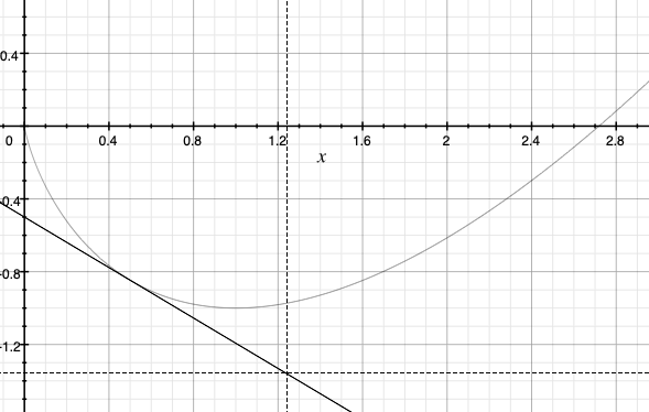 Here,
Here,
is the remainder term in the first-order Taylor-series expansion of the value of $F$ at $x$ when the expansion is carried out at \(x'\) and, for simplicity, we assume that \(F\) is differentiable on the interior of its domain \(\text{dom}(F) = \{ x\in \mathbb{R}\,:\, F(x)<+\infty \}\). Since for any convex function and any linear approximation of it stays below the graph of the convex function, we immediately get that \(D_F\) is nonnegative valued. For an illustration see the figure on the right, which shows a convex function, the first-order Taylor approximation of the function at some point.
One should think of \(F\) is a “nonlinear distance inducing function”; above \(D_F(x,x')\) can be thought of penalty imposed on deviating from \(x'\). However, \(D_F\) is more often than not is not a distance, i.e., often it is not even symmetric. Because of this, we can’t really call $D_F$ a distance. Hence, it is called a divergence. In particular, \(D_F(x,x')\) is called the Bregman divergence of \(x\) from \(x'\).
In the definition of the MD update rule, we tacitly assumed that \(D_F(x,x_{j-1})\) is well-defined. This requires that \(F\) should be differentiable at \(x_{j-1}\), which one needs to check when applying MD. In our specific case, this will hold, again.
The idea of the MD update rule is to (1) allow the learner to react to the last loss \(y_{j-1}\) vector chosen by the adversary, while also (2) limiting how much \(x_j\) can depart from \(x_{j-1}\), thus, effectively stabilizing the algorithm, the tradeoff governed by the choice of $\eta>0$. (Separating \(\eta\) from \(F\) only makes sense because there are some standard choices for \(F\), but \(\eta\) is really just a scale parameter for \(F\)). In particular, the larger the value of \(\eta\) is, the less “data-sensitive” MD will be (here, \(y_0,\dots,y_{k-1}\) constitute the data), and vice versa, the smaller \(\eta\) is, the more data-sensitive MD will be.
Where is the mirror?
Under some technical conditions on \(F\), the update rule \eqref{eq:mddef} has a two step-implementation:
\[\begin{align} \tilde x_j & = (\nabla F)^{-1} ( \nabla F (x_{j-1}) - \eta y_{j-1} )\,,\label{eq:mds1}\\ x_j &= \arg\min_{x\in \mathcal{X}} D_F(x,\tilde x_j)\,.\label{eq:mds2} \end{align}\]The first equation above explains the name: To obtain \(\tilde x_j\), one first transforms \(x_{j-1}\) using \(\nabla F: \text{dom}(\nabla F ) \to \mathbb{R}^d\) to the “mirror” (dual) space where “gradients”/”slopes live”, where one then adds to the result \(-\eta y_{j-1}\), which can be seen as a “gradient step” (interpreting \(y_{j-1}\) as the gradient of some loss). Finally, the result is then mapped back to the original (primal) space using the inverse of \(\nabla F\).
The second step of the update takes the resulting point \(\tilde x_j\) and “projects” it to \(\mathcal{X}\) in a way that respects the “geometry induced by \(F\)” on the space \(\mathbb{R}^d\).
The use of complex terminology, like “primal” and “dual” spaces, which happen to be the same old Euclidean space, \(\mathbb{R}^d\), probably sounds like an overkill. Indeed, in the simple case we consider when these spaces are identical it is. The distinction would become important when working with infinite dimensional spaces, which we leave to others for now.
Besides helping with understanding the terminology, the two-step update shown can also be useful for computation. In fact, this will be the case in the special case that we need.
Mirror descent on the simplex
We have seen that in the special case we need,
\[\begin{align*} \mathcal{X} &= \mathcal{P}_{d-1}:=\{ p\in [0,1]^{d}\,:\, \sum_a p_a = 1 \}\,, \\ \mathcal{Y} &= [-1/(1-\gamma),0]^d\,, \text{and} \\ d &= \mathrm{A}\,. \end{align*}\]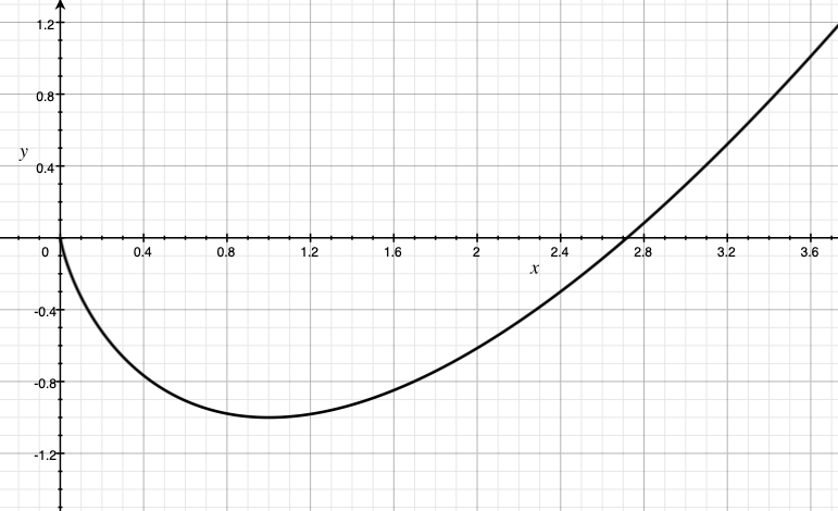 To use MD we need to specify the regularizer \(F\) and the learning rate. For the former, we choose
which is known as the unnormalized negentropy function. Note that \(F\) takes on finite values when \(x\in [0,\infty]^d\) (since \(\lim_{x\to 0+} x \log(x)=0\), we set \(x_i \log(x_i)=0\) whenever $x_i=0$). Outside of this quadrant, we define the value of \(F\) to be \(+\infty\). The plot of \(x\log(x)-x\) for \(x\ge 0\) is shown on the right.
It is not hard to verify that \(F\) is convex: First, \(\text{dom}(F) = [0,\infty]^d\) is convex. Taking the first derivative, we find that for any \(x\in (0,\infty)^d\),
\[\nabla F(x) = \log(x)\,,\]where \(\log\) is applied componentwise. Taking the derivative again, we find that for \(x\in (0,\infty)^d\),
\[\nabla^2 F(x) = \text{diag}(1/x)\,,\]i.e., the matrix whose $(i,i)$th diagonal entry is \(1/x_i\). Clearly, this is a positive definite matrix, which suffices to verify that \(F\) is a convex function.
The Bregman divergence induced by \(F\) is
\[\begin{align*} D_F(x,x') & = \langle \boldsymbol{1}, x \log(x) - x - x' \log(x')+x'\rangle - \langle \log(x'), x-x'\rangle \\ & = \langle \boldsymbol{1}, x \log(x/x') - x +x'\rangle \,, \end{align*}\]where again we use an “intuitive” notation when operations are first applied componentwise (i.e., $x \log(x)$ denotes a vector whose $i$th component is $x_i \log(x_i)$). Note that the domain of $D_F$ is \([0,\infty)^d \times (0,\infty)^d\). If both $x$ and $x’$ lie in the $d-1$-simplex, $D_F$ becomes the well-known relative entropy, or Kullback-Leibler (KL) divergence.
It is not hard to verify that $x_j$ can be obtained as shown in \eqref{eq:mds1}-\eqref{eq:mds2} and in particular this two-step update takes the form
\[\begin{align*} \tilde x_{j,i} &= x_{j-1,i} \exp(-\eta y_{j-1,i})\,, \qquad x_{j,i} = \frac{\tilde x_{j,i}}{ \sum_{i'} \tilde x_{j,i'}}\,, \quad i\in [d]\,. \end{align*}\]Unrolling the recursion, we can also that this is the same as
\[\begin{equation} \tilde x_{j,i} = \exp(-\eta (y_{0,i}+\dots + y_{j-1,i}))\,, \qquad x_{j,i} = \frac{\tilde x_{j,i}}{ \sum_{i'} \tilde x_{j,i'}}\,, \quad i\in [d]\,. \label{eq:mdunrolled} \end{equation}\]Based on this, it is obvious that MD can be efficiently implemented with this choice of $F$. As far as the regret is concerned, the following theorem holds:
Theorem (MD with negentropy on the simplex): Let \(\mathcal{X}= \mathcal{P}_{d-1}\) amd \(\mathcal{Y} = [0,1]^d\). Then, no matter the adversary, a learner using MD with
\[\eta = \sqrt{ \frac{2\log(d)}{k}}\]is guaranteed that its regret \(R_k\) in \(k\) rounds is at most
\[R_k \le \sqrt{2k \log(d)}\,.\]When the adversary plays in \(\mathcal{Y} = [a,b]^d\) with \(a<b\), we can use MD on the transformed sequence \(\tilde y_j = (y_j-b \boldsymbol{1})/(b-a) \in [0,1]^d\). Then, for any $x\in \mathcal{X}$,
\[\begin{align*} R_k(x) & := \sum_{j=0}^{k-1} \langle x_j-x, y_j \rangle \\ & = \sum_{j=0}^{k-1} \langle x_j-x, (b-a)\tilde y_j+b \boldsymbol{1} \rangle \\ & = (b-a)\sum_{j=0}^{k-1} \langle x_j-x, \tilde y_j \rangle \\ & \le (b-a) \sqrt{2k \log(d)}\,, \end{align*}\]where the third equality used that $\langle x_j,\boldsymbol{1}\rangle = \langle x, \boldsymbol{1} \rangle = 1$. Taking the maximum over $x\in \mathcal{X}$ gives that
\[\begin{align} R_k \le (b-a) \sqrt{2k \log(d)}\,. \label{eq:mdrbscaled} \end{align}\]By the update rule in \eqref{eq:mdunrolled},
\[\begin{align*} \tilde x_{j,i} = \exp(-\eta (\tilde y_{0,i}+\dots + \tilde y_{j-1,i})) = \exp(-\eta/(b-a) (y_{0,i}+\dots + y_{j-1,i}-j b) )\,, \qquad i\in [d]\,. \end{align*}\]Note that the “shift” by $-jb$ cancels out in the normalization step. Hence, MD in this case takes the form
\[\begin{equation} \begin{split} \tilde x_{j,i} &= \exp(-\eta/(b-a) (y_{0,i}+\dots + y_{j-1,i}))\,, \qquad x_{j,i} = \frac{\tilde x_{j,i}}{ \sum_{i'} \tilde x_{j,i'}}\,, \quad i\in [d]\,, \label{eq:mdunrolledscaled} \end{split} \end{equation}\]which is the same as before, except that the learning rate is scaled by $1/(b-a)$. In particular, in this case one can set
\[\begin{align} \eta = \frac{1}{b-a} \sqrt{\frac{2\log(d)}{k}}\,. \label{eq:etascaled} \end{align}\]and use update rule \eqref{eq:mdunrolled}.
MD applied to MDP planning
As agreed, \(T_1(s)\) from \eqref{eq:t1s} takes the form of a $k$-round regret against \(\pi^*(s,\cdot)\) in online linear optimization on the simplex with losses in \([-1/(1-\gamma),0]^{\mathrm{A}}\). This suggest to use MD in a state-by-state manner to control \(T_1(s)\). Using \eqref{eq:mdunrolled} and \eqref{eq:etascaled} gives
\[E_j(s,a) = \exp(\eta (\hat q_0(s,a) +\dots + \hat q_{j-1}(s,a)))\,, \qquad \pi_j(a|s) = \frac{E_j(s,a)}{ \sum_{a'} E_j(s,a')}\,, \quad a\in \mathcal{A}\]to be used with
\[\eta = (1-\gamma) \sqrt{\frac{2\log(\mathrm{A})}{k}}\,.\]Note that this is the update used by Politex. Then, \eqref{eq:mdrbscaled} gives that simultaneously for all $s\in \mathcal{S}$,
\[\begin{align} |T_1(s)| \le \frac{1}{1-\gamma} \sqrt{2k \log(\mathrm{A})}\,. \label{eq:t1sbound} \end{align}\]Putting things together, we get the following result:
Theorem (Politex suboptimality gap bound): Pick a featurized MDP $(M,\phi)$ with a full rank feature-map $\varphi: \mathcal{S}\times \mathcal{A} \to \mathbb{R}^d$ and let $K,m,H\ge 1$. Assume that B2\(_{\varepsilon}\) holds for $(M,\phi)$ and the rewards in $M$ are in the $[0,1]$ interval. For $0\le \zeta<1$, define
\[\kappa(\zeta) = \varepsilon (1 + \sqrt{d}) + \sqrt{d} \left(\frac{\gamma^H}{1 - \gamma} + \frac{1}{1 - \gamma} \sqrt{\frac{\log( d(d+1)K / \zeta)}{2m}}\right)\,,\]Then, in $K$ iterations, Politex produces a mixed policy $\bar \pi_K$ such that with probability $1-\zeta$, the suboptimality gap $\delta$ of $\bar \pi_K$ satisfies
\[\begin{align*} \delta \le \frac{1}{(1-\gamma)^2}\sqrt{\frac{2\log(\mathrm{A})}{K}}+\frac{2 \kappa(\zeta) }{1-\gamma} \,. \end{align*}\]In particular, for any $\varepsilon’>0$, choosing $K,H,m$ so that
\[\begin{align*} K & \ge \frac{32 \log(A)}{ (1-\gamma)^4 (\varepsilon')^2}\,, \\ H & \ge H_{\gamma,(1-\gamma)\varepsilon'/(8\sqrt{d})} \qquad \text{and} \\ m & \ge \frac{32 d}{(1-\gamma)^4 (\varepsilon')^2} \log( (d+1)^2 K /\zeta )\,, \end{align*}\]policy $\pi_K$ is $\delta$-optimal with
\[\begin{align*} \delta \le \frac{2(1 + \sqrt{d})}{1-\gamma}\, \varepsilon + \varepsilon'\,, \end{align*}\]while the total computation cost is $\text{poly}(\frac{1}{1-\gamma},d,\mathrm{A},\frac{1}{(\varepsilon’)^2},\log(1/\zeta))$.
Note that as compared to the result of LSPI with G-optimal design, the amplification of the approximation error $\varepsilon$ is reduced by a factor of $1/(1-\gamma)$, as it was promised. The price is that now the number of iterations $K$, is a polynomial of $\frac{1}{(1-\gamma)\varepsilon’}$, whereas before it was logarithmic. This suggest that perhaps a higher learning rate can help initially to speed up convergence to get the best of both words.
Proof: As in the proof of the suboptimality gap for LSPI, we get that for any $0\le \zeta \le 1$, with probability at least $1-\zeta$, for any $0 \le k \le K-1$,
\[\begin{align*} \| q^{\pi_k} - \hat q_k \|_\infty =\| q^{\pi_k} - \Pi \Phi \hat \theta_k \|_\infty \le \| q^{\pi_k} - \Phi \hat \theta_k \|_\infty &\leq \kappa(\zeta)\,, \end{align*}\]where the first inequality uses that \(q_{\pi_k}\) takes values in $[0,1]$. On the event when the above inequalities hold, by \eqref{eq:polsubgapgen} and \eqref{eq:t1sbound},
\[\begin{align*} \delta \le \frac{1}{(1-\gamma)^2}\sqrt{\frac{2\log(\mathrm{A})}{K}}+\frac{2 \kappa(\zeta) }{1-\gamma} \,. \end{align*}\]The details of this calculation are left to the reader. \(\qquad \blacksquare\)
Notes
Online convex optimization, online learning
Online linear optimization is a special case of online convex/concave optimization, where the learner chooses elements of some nonempty convex set \(\mathcal{X}\subset \mathbb{R}^d\) and the adversary needs to choose an element of a nonempty set \(\mathcal{Y}\) of concave functions over \(\mathcal{X}\): \(\mathcal{Y} \subset \{ f: \mathcal{X} \to \mathbb{R}\,:\, f \text{ is concave} \}\). Then, the definition of regret is changed to
\[\begin{align} R_k = \max_{x\in \mathcal{X}}\sum_{j=0}^{k-1} y_j(x) - y_j(x_j) \,, \label{eq:regretdefoco1} \end{align}\]where as before \(x_j\in \mathcal{X}\) is the choice of the learner for round \(j\) and \(y_j\in \mathcal{Y}\) is the choice of the adversary for the same round. Identifying any vector \(u\) of \(\mathbb{R}^d\) with the linear map \(x \mapsto \langle x, u \rangle\), we see that online linear optimization is a special case of this problem.
Of course, by negating all functions in \(\mathcal{Y}\) (i.e., letting \(\tilde {\mathcal{Y}} = \{ - y \,:\, y\in \mathcal{Y} \}\)) and redefining the regret to
\[\begin{align} R_k = \max_{x\in \mathcal{X}}\sum_{j=0}^{k-1} \tilde y_j(x_j)- \tilde y_j(x) \, \label{eq:regretdefoco} \end{align}\]we get a definition that is used in the literature, which prefers the convex case to the concave. Here, the interpretation is that \(\tilde y_j\in \tilde {\mathcal{Y}}\) is a “loss function” chosen by the adversary in round \(j\).
The standard function notation (\(y_j\) is applied to \(x\)) injects unwarranted asymmetry in the notation. After all, from the perspective of the learner, they need to choose a value in \(\mathcal{X}\) that works for the various functions in \(\mathcal{Y}\). Thus, we can consider any element of \(\mathcal{X}\) as a function that maps elements of \(\mathcal{Y}\) to reals through \(y \mapsto y(x)\). Whether \(\mathcal{Y}\) has functions in them or \(\mathcal{X}\) has functions in them does not matter that much; it is the interconnection between \(\mathcal{X}\) and \(\mathcal{Y}\) that matters more. For this reason, one can study online learning when \(y(x)\) above is replaced by \(b(x,y)\), where \(b: \mathcal{X}\times \mathcal{Y} \to \mathbb{R}\) is a specific map that assigns payoffs to every pair of points in \(\mathcal{X}\) and \(\mathcal{Y}\). When the map is fixed, one can spare an extra symbol by just using \([x,y]\) in place of \(b(x,y)\), which makes things almost a full circle given that we started with the linear case when \([x,y] = \langle x,y \rangle\).
Truncation or no truncation?
We introduced truncation to simplify the analysis. The proof can be made to go through even without it, with a mild increase of the suboptimality gap (or runtime). The advantage of removing the projection is that without projection, \(\hat q_0 + \dots + \hat q_{j-1} = \Phi (\hat \theta_0 + \dots + \hat \theta_{j-1})\), which leads to a practically significant reduction of the runtime.