7. Function Approximation

PDF Version

Our lower bound for online planners show that there are no online planners that lead to good policies in all MDPs while satisfying the following three requirements

the planner induces policies that achieve some positive fraction of the optimal value in all MDPs;
the per-state runtime shows polynomial dependence on the planning horizon $H$ and
it shows a polynomial dependence on the number of actions and
it shows no dependence on the number of states in the MDP.

Thus, one is left with no choice than to give up on one of the requirements. Since efficiency is clearly nonnegotiable (otherwise the runner just would not be practical), the only requirement that can be replaced is the first one. In what follows we will look at ways of relaxing this requirement.

In all the relaxations we will look at, we will essentially restrict the set of MDPs that the planner is expected to work on. However, we will do this in such a way that no MDP will be ever ruled out. We achieve this by giving the planner some extra hint about the MDP and we demand good performance only when the hint is correct. Since the hint will take a general form, some hint is always correct for any MDP. Hence, no MDP is left behind and the planner can again demanded to be efficient and effective.

Hints on value functions

The hints that we start with will concern the value functions. In particular, they state that either the optimal value, or the value function of all policies are effectively compressible.

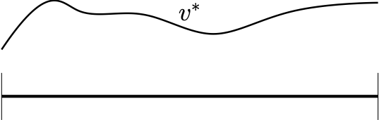drawing For motivation, consider the figure on the right. Imagine the state space is an interval of the real line and the optimal value function in an MDP looks like as shown on the figure: It is a nice, smooth function over the interval. As is well known, such relatively slowly changing functions can be well approximated by using the linear combination of a few fixed basis functions, like an appropriate polynomial, or Fourier basis, or using splines. Then, one hopes that even though the state space is large or even infinite as in this example, there could perhaps be a method that calculates the few coefficients needed get a good approximation to $v^*$ with a runtime that depends polynomially on the horizon, the number of actions and the number of coefficients that one needs to calculate. Given the knowledge of $v^*$ and simulator access to the MDP, good actions can then be efficiently obtained by performing one-step lookahead computations.

Linear function approximation

If the basis functions mentioned are $\phi_1,\dots,\phi_d: \mathcal{S} \to \mathbb{R}$ then, formally, the hope is that with some coefficients $\theta =(\theta_1,\dots,\theta_d)^\top\in \mathbb{R}^d$, we will have

\[\begin{align} v^*(s) = \sum_{i=1}^d \theta_i \phi_i(s)\, \qquad \text{for all } s\in \mathcal{S}\,. \label{eq:vstr} \end{align}\]

In the reinforcement learning literature, the vector $(\phi_1(s), \dots, \phi_d(s))^\top$ is called the feature vector assigned to state $s$. For a more compact notation we also use $\phi$ to be a map from $\mathcal{S}$ to $\mathbb{R}^d$ which assigns the feature vectors to the states:

\[\phi(s) = (\phi_1(s),\dots,\phi_d(s))^\top\,.\]

Conversely, given $\phi: \mathcal{S}\to \mathbb{R}^d$, its component are denoted using $\phi_1,\dots,\phi_d$. It will also be useful to introduce a matrix notation: Recall that the number of states is $\mathrm{S}$ and without loss of generality we may assume that $\mathcal{S} = [\mathrm{S}]$. Then, we can treat each of $\phi_1,\dots,\phi_d$ as $\mathrm{S}$-dimensional vectors: The $i$th component of $\phi_j$ is $\phi_j(i)$. Then, we can stack $\phi_1,\dots,\phi_d$ next to each other to form a matrix:

\[\Phi = \begin{pmatrix} | & | & \dots & | \\ \phi_1 & \phi_2 & \dots & \phi_d \\ | & | & \dots & | \end{pmatrix} \in \mathrm{R}^{\mathrm{S}\times d}\,.\]

That is, $\Phi$ is a $\mathrm{S}\times d$ matrix. The set of real-valued functions over the state space that can be described with the linear combination of the basis functions is

\[\mathcal{F} = \{ f: \mathcal{S} \to \mathbb{R} \,:\, \exists \theta\in \mathbb{R}^d \text{ s.t. } f(s) = \langle \phi(s),\theta \rangle \}\,.\]

Identifying the space of real-valued functions with the vector space $\mathbb{R}^{\mathrm{S}}$ in the natural way, $\mathcal{F}$ is a $d$-dimensional subspace of $\mathbb{R}^{\mathrm{S}}$, which is the same as the “column space”, or the span, or the range space of $\Phi$:

\[\mathcal{F} = \{ \Phi \theta \,:\, \theta\in \mathbb{R}^d \} = \text{span}(\Phi)\]

If we need to indicate the dependence of $\mathcal{F}$ on the choice of features, we will write either $\mathcal{F}_{\phi}$ or $\mathcal{F}_{\Phi}$.

Now, we have three equivalent ways of specifying the “features”, either by specifying the basis functions $\phi_1,\dots,\phi_d$, or the feature-map $\phi$, or the feature matrix $\Phi$, and we have a four equivalent way of specifying the functions that can be obtained via the linear combination of features.

Delivering the hint

Note that in the above problem description it is tacitly assumed that the feature-map, in some form or another, is available to the planner. In fact, the feature map can be made available in multiple ways. When we argue for lower bounds, especially for query complexity, we often assume that the whole feature-map is available for the algorithm. For upper bounds with online planning, the most natural assumption is that the planner gets from the simulator the feature vector of the states that it encounters. In particular, when it comes to online planning, the natural assumption is that the planner gets the feature vector of the initial state together with the state and with any subsequent calls to the simulator, the simulator returns the feature vector of the next states, together with the next states.

Typical hints

drawing In what follows we will study planning under a number of different hints (or assumptions) that connect the MDP and a feature-map. The simplest of this just states that $\eqref{eq:vstr}$ holds:

Assumption A1 ($v^*$-realizibility): The MDP $M$ and the featuremap $\phi$ are such that $v^* \in \mathcal{F}_\phi$

A second variation is when all value functions are realizable:

Assumption A2 (universal value function realizibility) The MDP $M$ and the featuremap $\phi$ are such that for any memoryless policy $\pi$ of the MDP, $v^\pi \in \mathcal{F}_\phi$.

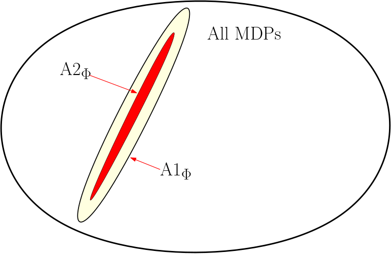
Clearly, A2 implies A1, because by the fundamental theorem of MDPs, there exists a memoryless policy $\pi$ such that $v^\pi = v^*$. The figure on the right illustrates the set of all finite MDPs with some state space and within those the set of those MDPs that satisfy A1 with a specific feature map $\phi$ (denoted by A1$\mbox{}_\phi$ on the figure), as well as those MDPs that satisfy A2 with the same feature map (denoted by A2$\mbox{}_\phi$). Both of these sets represent a very small fraction of all MDPs. However, of one changes the feature map, the union of all these sets clearly covers the set of all MDPs: The hint is general.

There are many variations of these assumptions. Often, we will find it useful to relax the assumption value functions are exactly realizable. Under the modified assumptions the value function does not need to lie in the span of the feature-map, but only in some vicinity of it. The natural error metric to be used is the maximum norm for reasons that will become clear later. To help with stating these assumptions in a compact form, introduce the notation

\[v\in_{\varepsilon} \mathcal{F}\]

to denote that

\[\inf_{f\in \mathcal{F}} \| f - v \|_\infty \le \epsilon\,.\]

That is, $v\in_{\varepsilon} \mathcal{F}$ means that the best approximator to $v$ from $\mathcal{F}$ approximates it within a uniform error of $\varepsilon$.

Fixing $\varepsilon\ge 0$ and replacing $\in$ with $\in_{\varepsilon}$ in the above two assumptions gives the following:

Assumption A1$\mbox{}_{\varepsilon}$ (approximate $v^*$ realizability): The MDP $M$ and the featuremap $\phi$ are such that $v^* \in_{\varepsilon} \mathcal{F}_\phi$

Assumption A2$\mbox{}_{\varepsilon}$ (approximate universal value function realizibility) The MDP $M$ and the featuremap $\phi$ are such that for any memoryless policy $\pi$ of the MDP, $v^\pi \in_{\varepsilon} \mathcal{F}_\phi$.

Action-value hints

We obtain new variants if we consider feature-maps that map state-action pairs to vectors. Concretely, (by abusing notation) let $\phi: \mathcal{S}\times\mathcal{A}\to \mathbb{R}^d$. Then, the analog of A1 is as follows:

Assumption B1 ($q^*$-realizibility): The MDP $M$ and the featuremap $\phi$ are such that $q^* \in \mathcal{F}_\phi$

Here, as expected, $\mathcal{F}_\phi$ is defined as the set of functions that lie in the span of the feature-map. The analog of A2 is as follows:

Assumption B2 (universal value function realizibility) The MDP $M$ and the featuremap $\phi$ are such that for any memoryless policy $\pi$ of the MDP, $q^\pi \in \mathcal{F}_\phi$.

We can also introduce positive approximation errors $\varepsilon>0$, which lead to B1$_{\varepsilon}$ and B2$_{\varepsilon}$:

Assumption B1$\mbox{}_{\varepsilon}$ (approximate $q^*$-realizibility): The MDP $M$ and the featuremap $\phi$ are such that $q^* \in_{\varepsilon} \mathcal{F}_\phi$

Assumption B2$\mbox{}_{\varepsilon}$ (approximate universal value function realizibility) The MDP $M$ and the featuremap $\phi$ are such that for any memoryless policy $\pi$ of the MDP, $q^\pi \in_{\varepsilon} \mathcal{F}_\phi$.

One may wonder why not choose one of these assumptions? When one assumption implies another, then clearly there is a preference to choose the weaker assumption. But often, there is going to be a price and sometimes the assumptions are just not comparable.

Notes

Origin

The idea of using value function approximation in planning dates back to at least the 1960s if not earlier. I include some intriguing early references at the end. That these ideas already appeared at the down of computing where computers hardly even existed is quite intriguing.

Infinite spaces

Function approximation is especially appealing when the state space, or the action space, or both are “continuous” (i.e., they are a subset of a Euclidean space). In this case, the compression is “infinite”. Experimental evidence suggests that function approximation can work quite well in the context of MDP planning in a surprisingly large number of different scenarios. When the spaces are infinite, all the “math” will still go through, except that occasionally one has to be a bit more careful. For example, one cannot clearly say that $\Phi$ is a matrix, but $\Phi$ can clearly be defined as a linear operator mapping $\mathbb{R}^d$ to the vector space of all real-valued functions over the (say) state space (when the feature map is also over states).

Where do the features come from?

It will be instructive to start with a special case. Low-rank MDPs are those where the transition kernel factorizes: For any $s,a,s’$ state-action-state triple,

\[P(s'|s,a) = \langle \phi(s,a), \nu(s') \rangle\]

for some $\phi: \mathcal{S}\times \mathcal{A} \to \mathbb{R}^d$ and $\nu(s’)\in \mathbb{R}^d$. If in addition to the above,

\[\begin{align} r(s,a) = \langle \phi(s,a), \nu' \rangle \label{eq:rfact} \end{align}\]

also holds for some $\nu’\in \mathbb{R}^d$, it is not hard to see that any action-value function lies in the space of the features $\phi$.

But what are the cases when the transition kernel factorizes? (If the transition kernel factorizes with some feature map $\phi_0$, one can always arrange for $\eqref{eq:rfact}$ to hold by adding an extra dimension to the feature map, filled with the values of the rewards.) A simple case is when state-action pairs can be clustered into non-overlapping groups such that for any two pairs $(s_1,a_1),(s_2,a_2)$ that belong to the same group, the transitions are identical: $P(\cdot|s_1,a_1) = P(\cdot|s_2,a_2)$. Assuming $d$ groups number from $1$ to $d$, $\phi_i(s,a)$ can be chosen as the indicator that $(s,a)$ belongs to the $i$th group ($i\in [d]$).

Another interesting case which leads to a factored transition kernel is when the state-space is $\mathbb{R}^p$ with some $p>0$ and the dynamics takes the form

\[S_{t+1} = f(S_t,A_t) + \eta_{t+1}\]

with some function $f$, and $(\eta_t)_t$ is a sequence of independent random variables with common density $g$. Then, the transition kernel takes the form $P(ds'|s,a) = g(s'-f(s,a)) ds'$. The important point here is that the noise introduced is homoscedastic (does not change with $(s,a)$). Take, for example, the case when $g(x) = \frac{1}{\sqrt{2\pi}} \exp(-x^2/2)$, i.e., $(\eta_t)_t$ are standard normal random variables. It is well known then that

\[g(x-y) = \langle u(x;\cdot,\cdot), u(y;\cdot,\cdot) \rangle\,,\]

where

\[u(x;\omega,b) = \sqrt{2} \cos(\omega^\top x + b )\]

and for $n,m: \mathcal{D} \to \mathbb{R}$, $\mathcal{D}:=\mathbb{R}^p \times [0,2\pi]$,

\[\langle n,m \rangle = \int_{\mathbb{R}^p}\, \frac{1}{2\pi} \int_0^{2\pi} n(\omega,b) m(\omega,b) \, \, db \, \prod_{i=1}^p g(\omega_i)\, d\omega \,.\]

From this, we get

\[P(ds'|s,a) = g(s'-f(s,a)) ds' = \langle u(s';\cdot,\cdot), u(f(s,a);\cdot,\cdot) \rangle ds'\,.\]

It follows that if we define $\phi: \mathcal{S}\times\mathcal{A} \to \mathbb{R}^{\mathcal{D}}$ via

\[(\phi(s,a))(\omega,b) = u(f(s,a);\omega,b)\]

then

\[P(ds'|s,a) = \langle \phi(s,a), u(s';\cdot,\cdot) \rangle ds'\,,\]

which is the same as above, except here $\phi$ is infinite dimensional. In a way, what happens here is that the noise introduces smoothness of the value functions. Smoothness of value functions can arise in some other ways. In the related topic of numerical computation of solutions of partial differential equations, Galerkin’s method also starts from assuming that the solution lies in the span of some features. In the relavant literature, various methods have been proposed to find appropriate features (or, basis functions, as they are called there). The book of Quarteroni et. al. gives several methods for automating the construction of these basis functions, and they also make a connection to optimal control.

Nonlinear value function approximation

The most successful use of the idea of compressing value functions uses neural networks. Readers are most likely are already familiar with the ideas underlying neural networks. The hope here is that whatever we find in the case of linear function approximation will have implications in how to use nonlinear function approximation in MDP planning. In a way, the very first question is whether one can decouple the design of the planning algorithm from what function approximation technique it is used with. We will study this question by asking for planners that work with any feature map. If we find that we can identify planners that are performant no matter the feature map, the decoupling is successful and we can hope that the ideas will generalize to nonlinear function approximation. However, if we find that successful planners need to use intricate properties of the feature maps, then this is must be taken as a warning that complications may arise when the results are generalized to nonlinear function approximation. In any case, it appears to be a prudent strategy to first investigate the simpler, more straightforward linear case, before considering the nonlinear case.

Computation with advice/Non-uniform Computation

Computation with advice is a general approach in computer science where a problem of computing a map is changed to computing a map which has an additional input, the advice. Clearly, the approach taken here can be seen as a special case of computation with advice. There is also the closely related notion of non-uniform computation studied in computability/complexity theory. In non-uniform computation, the Turing machine, in addition to its input, also receives some “advice” string.

References

The classical reference is a paper of Bellman et al. from 1963, where they proposed to use linear function approximation in a specific context for approximating the optimal value functions (Bellman et al. 1963). Other early papers are by Daniel (1976) and Schweitzer and Seidmann (1985). In the latter paper, the authors generalized the earlier constructions of Bellman and others and, with modern terminology, they introduced fitted value iteration, fitted policy iteration and approximate linear programming as possible approaches.

The observation that homoscedastic noise makes it so that the transition kernel factorizes is due to Ren et al. (2022). The book of Quarteroni et al. (2016) describes various methods for automating the construction of basis functions for the solution of parametric family of partial differential equations.

Richard Bellman, Robert Kalaba and Bella Kotkin. 1963. Polynomial Approximation–A New Computational Technique in Dynamic Programming: Allocation Processes. Mathematics of Computation, 17 (82): 155-161
Daniel, James W. 1976. “Splines and Efficiency in Dynamic Programming.” Journal of Mathematical Analysis and Applications 54 (2): 402–7.
Schweitzer, Paul J., and Abraham Seidmann. 1985. “Generalized Polynomial Approximations in Markovian Decision Processes.” Journal of Mathematical Analysis and Applications 110 (2): 568–82.
Brattka, Vasco, and Arno Pauly. 2010. Computation with Advice. arXiv [cs.LO].
Quarteroni, Alfio, Andrea Manzoni, and Federico Negri. “Reduced Basis Methods for Partial Differential Equations”. Springer International Publishing. 2016.
Ren, T., T. Zhang, C. Szepesvári, and B. Dai. 2022. “A Free Lunch from the Noise: Provable and Practical Exploration for Representation Learning.” UAI. abstract