10. Planning under $q^*$ realizability
The lesson from the last lecture is that efficient planners are limited to induce policies whose suboptimaly gap is polynomially larger than the misspecification error of the feature-map supplied to the planner. We have also seen) that if we accept this polynomial in the feature-space-dimension error amplification, a relatively straightforward adaptation of policy iteration gives rise to a computationally efficient (global) planner – at least, when the planner is furbished with the solution to an underlying optimal experimental design problem. In any case, the planner is query efficient.
All this was shown in the context when the misspecification error is relative to the set of action value functions underlying all possible policies. In this lecture we look into whether this error metric could be changed so that the misspecification error is measured by how well the optimal action-value function, $q^*$, is approximated by the features, while still retaining the positive result. As the negative result already implies that there are no efficient planners unless the suboptimality gap of the induced policy is polynomially larger than the approximation error, we look into the case when the optimal action-value function is perfectly representable with the features supplied to the planner. This assumption is also known as “\(q^*\)-realizability”, or, “\(q^*\) linear realizability”, if we want to be more specific about the nature of the function approximation technique used.
Planning under \(q^*\) realizability
We consider fixed horizon online planning in large finite MDPs $(\mathcal{S},\mathcal{A},P,r)$. As usual, the horizon is denoted by $H>0$ and we consider planning with a fixed initial state $s_0$, as in the previous lecture. Let us denote by \(\mathcal{S}_i\) the states that are reachable from $s_0$ in $0\le i \le H$ steps. As before, we assume that \(\mathcal{S}_i\cap \mathcal{S}_j=\emptyset\) when $i\ne j$. Recall that in this case the action-value functions depend on the number of steps left, of the current stage. For a fixed $0\le h\le H-1$, let \(q^*_h:\mathcal{S}_{h} \times \mathcal{A}\to \mathbb{R}\) be the optimal action-value function with $h$ stages in the process, $H-h$ stages left. Since we do not need the values of $q^*_h$ outside of $\mathcal{S}_h\times \mathcal{A}$, we abuse notation by redefining it restricted to this set.
Important note: The indexing of $q^*_h$ used here is not consistent with the indexing used in the previous lecture, where it was more convenient to index value functions based on the number of stages left.
The planner will be given a feature map $\phi_h$ for every stage $0\le h\le H-1$ such that \(\phi_h:\mathcal{S}_h \times \mathcal{A} \to \mathbb{R}^d\). The realizability assumption means that
\[\begin{align} \inf_{\theta\in \mathbb{R}^d} \max_{0\le h \le H-1}\|\Phi_h \theta - q^*_{h} \|_\infty = 0\,. \label{eq:qsrealizability} \end{align}\]Note that we demand that the same parameter vector is shared between all stages. As it turns out, this makes our result stronger. Regardless, at the price of increasing the dimension from $d$ to $dH$, one can always assume that the parameter vector is shared. Since we will give a negative result concerning the query-efficiency of planners, we allow the planners access to the full feature-map: The negative result still applies even if the planner is allowed to perform any sort of computation with the feature-map during or before the planning process.
For $\delta>0$, we call an online planner $\delta$-sound for the $H$-step criterion if for any MDP $M$ and feature map $\phi = (\phi_h)_h$ pair such that the optimal action-value function of $M$ is realizable with the features $\phi$ in the sense that \eqref{eq:qsrealizability} holds, the planner induces a policy that is $\delta$-suboptimal or better when evaluated with the $H$-horizon undiscounted total reward criterion from the designated start-state \(s_0\) in MDP $M$. Note that this is very much the same as the previous $(\delta,\varepsilon=0)$ soundness criterion, except that the definition of the approximation error is relaxed, while we demand $\varepsilon=0$.
The result below uses MDPs where the immediate reward (obtained from the simulator) can be random. The random reward is used to make the job of the planners harder and it allows us to consider MDPs with deterministic dynamics. (The result could also be proven for MDPs with deterministic rewards and random transitions.)
The usual definition of MDPs with random transitions and rewards is in a way even simpler: Such a (finite) MDP is given by the tuple \(M=(\mathcal{S},\mathcal{A},Q)\) where \(Q = (Q_a(s))_{s,a}\) is a collection of distributions over state-reward pairs. In particular, for all state-action pairs $(s,a)$, \(Q_a(s)\in \mathcal{M}_1(\mathcal{S}\times\mathbb{R})\). Letting \((S',R)\sim Q_a(s)\) (i.e., $(S’,R)$ is drawn from \(Q_a(s)\) at random), we can recover $P_a(s)$ as the distribution of $S’$ and $r_a(s)$ as the expected value of $R$. That the reward can be random forces a change to the notion of the canonical probability spaces, since histories now also show include rewards, $R_0,R_1,\dots$ incurred in each time step $t=0,1,\dots$. With appropriate modifications, we can nevertheless still introduce \(\mathbb{P}_\mu^\pi\) and the corresponding expectation operator, \(\mathbb{E}_\mu^\pi\), as well. The natural definition of the value of a policy $\pi$ at state $s$, say, in the discounted setting is then \(v^\pi(s) = \mathbb{E}_s^\pi[ \sum_{t=0}^\infty \gamma^t R_t]\). However, it is easy to see that for any $t\ge 0$, \(\mathbb{E}_\mu^\pi[R_t]=\mathbb{E}_\mu^\pi[r_{A_t}(S_t)]\), and, as such, nothing changes in the theoretical results derived so far.
For $a,b$ reals, let $a\wedge b = \min(a,b)$. The main result of this lecture is as follows:
Theorem (worst-case query-cost is exponential under $q^*$-realizability): For any $d,H$ large enough and any online planner $\mathcal{P}$ that is $9/128$-sound for the $H$-horizon planning problem, there exists a triplet $(M,s_0,\phi)$ where $M$ is a finite MDP with random rewards taking values in $[0,1]$ and deterministic transitions, $s_0$ is a state of this MDP and $\phi$ is a $d$-dimensional feature-map such that \eqref{eq:qsrealizability} holds for the optimal action-value function \(q^* = (q^*_h)_{0\le h \le H-1}\) and the expected number of queries $q$ that $\mathcal{P}$ uses when interconnected with $(M,s_0,\phi)$ satisfies
\[q = e^{\Omega(d\wedge H )}\]Note that with random rewards with no control on their tail behavior (e.g., unbounded variance) it would not be hard to make the job of any planner arbitrarily hard. As such, it is quite important that the MDPs that are constructed for the result, the rewards, while random, lie in a fixed interval. Note that the specific choice of this interval does not matter: If there is a hard example with some interval, that example can be translated into another by shifting and scaling, and at the price of introducing an extra dimension in the feature map to account for the shifts. A similar comment applies to $\delta = 9/128$ (which, nevertheless, needs to be scaled to the range of the rewards).
The main ideas of the proof
 Rather than giving the full proof, we will just explain the main ideas behind it. At a high-level, the proof merges the ideas behind the lower bound for the small action-set case and the lower bound of the large action-set case. That is, we will consider an action set that is exponentially large in $d$. In particular, we will consider action sets that have $k=e^{\Theta(d)}$ elements.
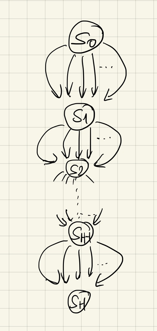
Note that because realizability holds, having a large action set but with a trivial dynamics (as in the lower bound in the last lecture) does not lead to the lower bound of the desired form. In particular, if the dynamics are trivial (i.e., $\mathcal{S}_i={s_i}$, see the figure on the right) then the optimal action to be taken at $s_0$ does not depend on what actions are taken at later stages and can be efficiently found by just maximizing for the reward received in that stage, which can be done efficiently due to our realizability assumption, even in the presence of random rewards. Whether an example exists with only a few actions but with a more complicated dynamics remains open. With the construction provided here (which is based on tree dynamics and zero intermediate reward in the tree), this clearly fails, as we will make it clear below.
In any case, since the “chain dynamics” does not work, the next simplest approach is to have a tree, but with exponentially many actions in every node. Since this creates many many states ($e^{\Theta(dh)}$ states at stage $h$) the next question then is how to ensure realizability. There are two issues: We need to be able to keep the dimension fixed at $d$ at every stage and somehow we will need to have a way of controlling which action should be optimal at each state at each stage. Indeed, realizability means that we need to ensure that for all $0\le h \le H-1$ and $(s,a)\in \mathcal{S}_h \times \mathcal{A}$,
\[\begin{align} q_{h}^*(s,a) = r_a(s)+v_{h+1}^*(sa) \label{eq:cons} \end{align}\]Here, $sa$ stands for the state that is reached by taking action $a$ in state $s$ (in the tree, every node, or state is uniquely indexed by the action sequence that reaches it). Now, in the definition of $v_{h}^*$, for all $h$, we also have \(v_{h}^*(s) = \max_{a\in \mathcal{A}} q_{h+1}^*(s,a)\), which calls for the need to know the identity of the maximizing action. What is more, since the solution to the Bellman optimality equations is unique, if we guarantee that \eqref{eq:cons} holds at all state-action pairs for \(q_h(s,a) = \langle \phi_h(s,a), \theta^* \rangle\) with some features and parameter vectors, it also follows that \(q_h = q^*_h\) for all \(h\ge 0\), that is, \(q^*\) is realizable with the features.
A simple approach to resolve all of these issues is to let a fixed action $a^*\in \mathcal{A}$ be the optimal action at all the states, together with using the JL features from the previous lecture (the identity of this action is of course hidden from the planner). In particular, the JL feature-matrix lemma from the previous lecture furnishes us with $k$ $d$-dimensional unit vectors $(u_a)_{a\in \mathcal{A}}$ such that for $a\ne a’$,
\[\begin{align*} \vert \langle u_a, u_a' \rangle \vert \le \frac{1}{4}\,. \end{align*}\]Fix these vectors. That $a^*$ should be optimal at all states $s$ is equivalent to that
\[\begin{align} q_h^*(s,a)\le q_h^*(s,a^*) (=v_h^*(s)), \qquad 0\le h \le H-1, s\in \mathcal{S}_h, a\in \mathcal{A}\,. \label{eq:aopt} \end{align}\]In our earlier proof we used \(\phi_h(s,a) = u_a\) and \(\theta^* = u_{a^*}\). Will this still work? Unfortunately, it does not. The first observation is that from this it follows that for any $h$, $s$, $a$,
\[\begin{align*} q_{h}^*(s,a) = \langle u_{a^*}, u_a \rangle\,. \end{align*}\]As such, for almost all the actions $a$, we expect \(|q_h^*(s,a)|\) to be close to \(1/4\). Now, under this choice we also have that \(v_h^*(s)=1\) for all states and all stages $0\le h \le H-1$. This creates essentially the same problem as what we saw above with the trivial chain dynamics. In particular, from \eqref{eq:cons} we get that \(q_h^*(s,a) = r_a(s)+1\). As such, we expect $r_a(s)$ to be close to either $-3/4$ or $-5/4$ (since \(|q_h^*(s,a)|\) is close to $1/4$). Putting aside the issue that we wanted the immediate reward be in $[0,1]$, we see that if the reward noise is not large, \(\theta^*\) and thus the identity of $a^*$ can be obtained with just a few queries: The signal to noise ratio is just too good!
This problem replicates itself at the very last stage: Here, \(v_H^*(s')=0\) for any state $s’$, hence
\[\begin{align} q^*_{H-1}(s,a)=r_a(s) \label{eq:laststage} \end{align}\]for any $(s,a)$ pair. Unless we choose \(q^*_{H-1}(s,a)\) to be small, say, \(e^{-\Theta(H)}\), a planner will succeed with fewer queries than in our desired bound.
This motivates us to introduce a scaling of the features (recall that the parameter vector is shared between the stages) with some scaling factors. For maximum generality, we allow for the scaling factor of the feature vector of \((s,a)\in \mathcal{S}_h\times \mathcal{A}\) to depend on \((s,a)\) itself (since states between stages are not shared, scaling can depend on the stage with this choice). Let \((3/2)^{-h+1}\sigma_{sa}\) be the scaling factor we intend to use with \((s,a)\) where we intend to keep $\sigma_{sa}$ in a constant range (so the scaling with the stage index works as intended) while we aim to use \(\phi_h(s,a) =(3/2)^{-h+1} \sigma_{sa} u_a\).
Now, we can explain the need for many actions. By the Bellman optimality equation \eqref{eq:cons} we have that for any suboptimal action, $a$,
\[r_{a^*}(s)-r_a(s) =q_h^*(s,a^*)-q_h^*(s,a) \approx (3/2)^{-h} \langle u_{a^*}-u_a,u_{a^*} \rangle \ge (3/2)^{-h} (3/4),\]where \(\approx\) uses that \(\sigma_{sa}\approx\sigma_{sa^*}\approx \text{const}\). From this we see that close to the initial state \(s_0\) the reward gaps are of constant order. In particular, if there were only a few actions per state, a planner could identify the optimal action by finding the action whose reward is significantly larger than that of the others. By choosing to have many actions, the planner faces a “needle-in-a-haystack” situation, which makes their job hopeless even with perfect signal (no noise).
The next idea is to force “clever” planners to only experiment with actions in the last stage. Since here, the signal-to-noise ratio will be very poor, if we manage to achieve this, even clever planners will need to use a large number of queries. A simple way of forcing this is to choose all the rewards while transitioning in the tree and taking suboptimal actions to be identically zero except for stage $h=H-1$, where, in accordance to our earlier plan, the rewards are chosen at random to ensure consistency but the signal to noise ratio will be poor.
Since the dynamics in the tree is known, and it is known that all rewards are zero with the possible exception of when using the optimal action (one of exponentially many actions and is thus hard to find), planners are either left with either solving the needle in a haystack problem of identifying the optimal action by randomly stumbling upon it, or they need to experiment with actions in the last stage. That the rewards are chosen to be identically zero is not critical: From the point of view of this argument, what is critical is that they are all the same.
It remains to be seen that consistency can be achieved and also that the optimal action at $s_0$ has a large value compared to the values of suboptimal actions at the same state. Here, we still face some challenges with consistency. Since we want the immediate rewards to belong to the $[0,1]$ interval, all the action values have to be nonnegative. As such, it will be easier if we introduce an additional bias component $c_h$ in the feature vectors, which we allow to scale with the stage.
To summarize, we let
\[\begin{align*} \phi_h(s,a) = ( c_h, (3/2)^{-h+1} \sigma_{sa} u_a^\top )^\top\,. \end{align*}\]while we propose to use
\[\begin{align*} \theta^* = \frac{1}{3} (1, u_{a^*}^\top)^\top \,. \end{align*}\]It remains to show that \eqref{eq:aopt} and \eqref{eq:cons} can be satisfied with \(q_h(s,a):=\langle \phi_h(s,a), \theta^* \rangle\), while also keeping the suboptimal gap of \(a^*\) at \(s_0\) large, and while the last stage rewards (\eqref{eq:laststage}) are in $[0,1]$ and are of size \(e^{-\Theta(H)}\) as planned.
Assume for a moment that \(a^*\) is optimal in all states, i.e., that \eqref{eq:aopt} holds. Then, \(a^*\) is also optimal in state $sa$, hence, under \(q^*_h=q_h\), \eqref{eq:cons} for any \(a\ne a^*\) is equivalent to
\[\begin{align*} q_h(s,a) = q_{h+1}(sa,a^*) \end{align*}\]where we also used that by assumption $r_a(s)=0$ because \(a\ne a^*\). Plugging in the definitions,
\[\begin{align} \sigma_{sa,a^*} = \left(\frac{3}{2}\right)^h \left(c_h-c_{h+1}\right) + \frac{3}{2} \sigma_{sa} \langle u_a,u_{a^*} \rangle\,. \label{eq:sigmarec} \end{align}\]Define \((c_h)_{0\le h\le H-1}\) so that
\[\begin{align*} \left(\frac{3}{2}\right)^h \left(c_h-c_{h+1}\right) =\frac{5}{8}\,. \end{align*}\]with \(C_{H-1} = \frac{1}{2}\left(\frac32\right)^{-H}\) (i.e., $c_h$ is a decreasing geometric sequence) This has two implications: \eqref{eq:sigmarec} simplifies to
\[\begin{align} \sigma_{sa,a^*} = \frac{5}{8} + \frac{3}{2} \sigma_{sa} \langle u_a,u_{a^*} \rangle\,, \label{eq:sigmarec2} \end{align}\]and also for the last stage rewards, from \eqref{eq:laststage} we get
\[\begin{align*} r_a(s) = \frac{1}{3} \left(\frac32\right)^{-H} \left( \frac{1}{2} + \sigma_{sa} \frac32 \langle u_a,u_{a^*}\rangle\right)\,. \end{align*}\]Clearly, if $\sigma_{sa}\in [-4/3,4/3]$, since for \(a\ne a^*\), \(\vert \langle u_a,u_{a^*}\rangle \vert \le 1/4\), \(r_a(s)\in [0,(3/2)^{-H}/3]\) while also \(r_{a^*}(s)\in [0,1]\).
With this, to satisfy \eqref{eq:cons}, on the one hand we choose to define $\sigma_{sa}$ with the following “downward recursion” in the tree: For any $s$ in the tree and actions $a,a’$,
\[\begin{align} \sigma_{sa,a'} = \frac{5}{8} + \frac{3}{2} \sigma_{sa} \langle u_a,u_{a'} \rangle\,. \label{eq:sigmarec3} \end{align}\]Note that this is consistent with \eqref{eq:sigmarec2}. The next challenge is to show that $\sigma_{sa}$ stays within a constant range. In fact, with the above definition, this will not hold. In particular, when $a=a’$, the right-hand side can be as large as \(5/8+3/2 \sigma_{sa} \ge 3/2 \sigma_{sa}\), which means that the scaling coefficients will exponentially increase with a base of $(3/2)$. Note, however, that if $a\ne a’$, then provided that \(\sigma_{sa}\in [1/4,1]\) (which can be ensured at the root by choosing \(\sigma_{s_0,a}=1\) for all actions \(a\)),
\[\frac{1}{4} = \frac{5}{8} - \frac{3}{8} \le \frac{5}{8} + \frac{3}{2} \sigma_{sa} \langle u_a,u_{a'} \rangle \le \frac{5}{8} + \frac{3}{8} \le 1\,,\]and thus \(\sigma_{sa,a'}\in [1/4,1]\) will also hold.
Hence, we modify the construction so that the definition \eqref{eq:sigmarec3} is never needed for $a=a’$. This is achieved by changing the dynamics: We introduce a special set of states, ${e_1,\dots,e_H}$, the exit lane. Once, the process gets into this lane, there is now return and in fact all the remaining rewards up the end are zero. Specifically, all the actions in $e_h$ lead to state $e_{h+1}$ and we set the feature vector of all states in the exit-lane zero:
\[\phi_h(e_h,a) = \boldsymbol{0}\,.\]This way, regardless the choice of the parameter vector, we ensure that the Bellman optimality equations hold at these state and the optimal values are correctly set to zero.
The exit lane is introduced to remove the need to use \eqref{eq:sigmarec3} with repeat actions. In particular, for any \(s\in \mathcal{S}_h\) with some $h\ge 1$, say, \(s=(a_1,\dots,a_h)\) (i.e., $s$ is obtained by following these actions) then if for \(a\in \{a_1,\dots,a_h\}\), the next state is $e_{h+1}$. Since the optimal value of $e_{h+1}$ is zero and we don’t intend to introduce an immediate reward, we set
\[\phi_h(s,a)=\boldsymbol{0}\,,\]making the value of repeat actions zero. The next complication is that this ruins our plan to keep \(a^*\) optimal at all states: Indeed, \(a^*\) could be applied multiply times in a path from \(s_0\) to a leaf of the tree, and by the second application, the new rule forces the value of \(a^*\) to be zero. Hence, we need to modify this rule when the action is \(a^*\).
Clearly, whether a suboptimal action, or \(a^*\) is repeated is problematic for the recursive definition of $\sigma_{sa}$. Hence, it is better if \(a^*\) is also forced to use the exit lane. Thus, if \(a^*\) is used in \(s\in \mathcal{S}_h\) with \(h\ge 0\), the next state is \(e_{h+1}\). However, we do not zero out \(\sigma_{sa^*}\), but keep the recursive definition and we rather introduce an immediate reward to match \(q_h(s,a^*) = \langle \phi_h(s,a^*), \theta^* \rangle\). It is not hard to check that this reward is also in the \([0,1]\) range. Note that here if \(s = (a_1,\dots,a_h)\) then by definition \(a^*\not\in \{a_1,\dots,a_h\}\). This completes the description of the structure of the MDPs.
That the action gap at \(s_0\) is large follows from the choice of the JL feature vectors.
It remains to be seen that \(a^*\) is indeed the optimal action at any state. This boils down to checking that for \(a'\ne a^*\), \(q_{h+1}(sa,a^*)-q_{h+1}(sa,a')\ge 0\). When \(a'\) is a repeat action, this is trivial. When \(a'\) is not a repeat action, we have
\[q_{h+1}(sa,a^*)-q_{h+1}(sa,a') = \frac{1}{3}\left(\frac{3}{2}\right)^{-h} \left[ \sigma_{sa,a^*}-\sigma_{sa,a'}\langle u_{a'},u_{a^*}\rangle \right] \ge \frac{1}{3}\left(\frac{3}{2}\right)^{-h} \left[ \frac{1}{4}-\frac{1}{4} \right] = 0\]where we used that \(\sigma_{sa,a^*}\ge 1/4\) and \(1/4\le \sigma_{sa,a'}\le 1\) and thus \(\sigma_{sa,a'}\langle u_{a'},u_{a^*}\rangle\ge -\frac{1}{4}\) by the choice of \((u_a)_a\) and since \(a\ne a'\).
Let \(M_{a^*}\) denote the MDP constructed this way when the optimal action is \(a^*\) (the feature maps, of course, are common between these MDPs). For a formal proof, one also needs to argue that planners that do not use many queries cannot distinguish between these MDPs. Intuitively, this is because such planners will receive, with high probability, identical observations under different MDPs in this class. As such, these planners can at best randomly choose an action (“needle in a haystack”) and since in MDP \(M_{a}\) only action \(a\) incurs high values, they cannot induce a policy with a near-optimal value.
Computation with many actions
In the construction given the number of actions was allowed to scale exponentially with the dimension. The above proof would show a separation between the query and computation complexity of planning, if one could demonstrate that there is a choice of the JL feature vectors when the optimization problems
\[\begin{align*} \arg\max_{a\in \mathcal{A}} \langle \phi(s,a), \theta \rangle \end{align*}\]admits a computationally efficient solver regardless of the choice of $\theta\in \mathbb{R}^d$ and $s\in \mathcal{S}$ (for simplicity, we suppress dependence on $h$). Whether such a solver exist will depend on the choice of the feature-map and this is a fascinating question on its own. One approach to arrive at such a solver is to rewrite this problem as the problem of finding
\[\begin{align} \arg\max_{v\in V_s} \langle v, \theta \rangle \label{eq:linopt} \end{align}\]where $V_s \subset \mathbb{R}^d$ is the convex hull of the feature vectors \(\{ \phi(s,a) \}_{a\in \mathcal{A}}\). Provided that this problem admits an efficient solution and given any extreme point of $v\in V_s$, we can efficiently recover an action $a\in \mathcal{A}$ such that $\phi(s,a)=v$ (this amounts to “inverting” the feature map), the first problem can also be solved efficiently.
Note that \eqref{eq:linopt} is a linear optimization problem over a convex set $V_s$ and the question whether this problem admits an efficient solver lies at the heart of computer science. The general lesson is that the answer can be expected to be yes when $V_s$ has some “convenient” description other than the one that is used to define it. The second problem of inverting the feature map is known as the “decomposition problem” and the same conclusions hold for this problem.
Notes
-
It is possible to modify the construction to make it work in the discounted setting. The paper cited below shows how.
-
Back to the finite horizon setting, for an upper bound, one can employ the least-squares value iteration algorithm with $G$-optimal design (LSVI-G), which we have met in Homework 2. What results is that to get a $\delta$-sound (global) planner with this approach,
queries are sufficient (and the compute cost is also of similar order). We see that as far as the exponents in the lower and upper bounds are concerned, in the upper bound the exponent is \(\Theta(H \log_2(d))\) while in the lower bound it is \(O(H\wedge d)\). Thus, there remains a logarithmic gap between them when $H\ll d$, while the gap is unbounded when \(H \gg d\), i.e., for long horizon problems. In particular, in the constant dimension and long-horizon featurized planning problem, the LSVI-G algorithm seems to be suboptimal because it calculates the optimal action-value function stage-wise. One conjectures that the upper bound for LSVI-G is tight, while the lower bound in this lecture is also essentially correct. This would means that there is an alternate algorithm that could perform much better than LSVI-G in large-horizon planning with constant feature-dimension. Clearly, for the specific construction used in this lecture, a planner that tries all actions, say at \(s_0\), will find the optimal action and the cost of this planner is independent of the horizon. Hence, at least in this case, the lower bound can be matched with an alternate algorithm. One may think that this problem is purely of theoretical interest. To counter this note that long-horizon planning is a really important practical question: Many applications require thousands of steps, if not millions, while perhaps the feature space dimension does not need to be very large. Whether there exist an algorithm that works better than LSVI-G thus remains to be a fascinating open problem with good potential for having a real impact on applications.
- For infinite horizon undiscounted problems and \(v^*\) realizability, there is a simple example that shows that with \(\Theta(d)\) actions and $d$-dimensional features, any query efficient planner that guarantees a constant suboptimality gap needs \(\Omega(2^d/d)\) queries per state. This is based on a shortest path problem on a regular grid. Here, the obstruction is simply algebraic: There is no noise in either the transitions or the rewards.
Bibliographical notes
This lecture is entirely based on the paper
- Weisz, Gellert, Philip Amortila, and Csaba Szepesvári. 2020. “Exponential Lower Bounds for Planning in MDPs With Linearly-Realizable Optimal Action-Value Functions.”,
which is available on arXiv and which will also soon appear at ALT.
The second lower for the undiscounted setting mentioned in the notes is from
- Weisz, Gellert, Philip Amortila, Barnabás Janzer, Yasin Abbasi-Yadkori, Nan Jiang, and Csaba Szepesvári. 2021. “On Query-Efficient Planning in MDPs under Linear Realizability of the Optimal State-Value Function.”
available on arXiv.
A beautiful book that is a very good source on reading about the linear optimization problem mentioned above is
- Grotschel, Martin, László Lovász, and Alexander Schrijver. 1993. Geometric Algorithms and Combinatorial Optimization. Vol. 2. Algorithms and Combinatorics. Berlin, Heidelberg: Springer Berlin Heidelberg.