8. Approximate Policy Iteration
Note: On March 13, 2021, these notes were updated as follows:
- Tighter bounds are derived; the old analysis was based on bounding \(\| q^*-q^{\pi_k} \|_\infty\); the new analysis directly bounds \(\| v^* - v^{\pi_k} \|_\infty\), which leads to a better dependence on the approximation error;
- Unbiased return estimates are introduced that use rollouts of random length.
One simple idea to use function approximation in MDP planning is to take a planning method that uses internal value functions and add a constraint that restrict the value functions to have a compressed representation.
As usual, two questions arise:
- Does this lead to an efficient planner? That is, can the computation be carried out in time polynomial in the relevant quantities, but not the size of the state space? In the case of linear functions the question is whether we can calculate the coefficients efficiently.
- Does this lead to an effective planner? In particular, how good a policy can we arrive at with a limited compute effort?
In this lecture, as a start into exploring the use of value function approximation in planning, we look at modifying policy iteration in the above described way. The resulting algorithm belongs to the family of approximate policy iteration algorithms, which consists of all algorithms derived from policy iteration by adding approximation to it.
We will work with linear function approximation. In particular, we will assume that the planner is given as a hint a feature-map $\varphi: \mathcal{S}\times \mathcal{A}\to \mathbb{R}^d$. In this setting, since policy iteration hinges upon evaluating the policies obtained, the hint given to the planner is considered to be “good” if the (action-)value functions of all policies are well-represented with the features.
This means, that we will work under assumption B2$_\varepsilon$ from the previous lecture, which we copy here for convenience. In what follows we fix $\varepsilon>0$.
Assumption B2$\mbox{}_{\varepsilon}$ (approximate universal value function realizibility) The MDP $M$ and the featuremap $\varphi$ are such that for any memoryless policy $\pi$ of the MDP, \(q^\pi \in_{\varepsilon} \mathcal{F}_\varphi\).
Recall that here the notation $q^\pi \in_{\varepsilon} \mathcal{F}_\varphi$ means that $q^\pi$ can be approximated up to a uniform error of $\varepsilon$ using linear combinations of the basis functions underlying the feature-map $\varphi$:
For any policy $\pi$,
\[\begin{align*} \inf_{\theta\in \mathbb{R}^d} \max_{(s,a)} | q^\pi(s,a) - \langle \theta, \varphi(s,a) \rangle | \left(= \inf_{\theta\in \mathbb{R}^d} \| q^\pi - \Phi\theta \|_\infty\right) \le \varepsilon\,. \end{align*}\]One may question whether it is reasonable to expect that the value functions of all policies can be compressed. We will come back to this question later.
Approximate Policy Evaluation: Done Well
Recall that in phase $k$ of policy iteration, given a policy $\pi_k$, the next policy $\pi_{k+1}$ is obtained as the policy that is greedy with respect to $q^{\pi_k}$. If we found some coefficients $\theta_k\in \mathbb{R}^d$ such that
\[\begin{align*} q^{\pi_k} \approx \Phi \theta_k\,, \end{align*}\]then when it comes to “using” policy $\pi_{k+1}$, we could just use $\arg\max_{a} \langle \theta_k,\varphi(s,a)\rangle$ when an action is needed at state $s$. Note that this action can be obtained at the cost of $O(d)$ elementary operations, a small overhead compared to a table lookup (with idealized $O(1)$ access times).
Hence, the main question is how to obtain this parameter in an efficient manner. To be more precise, here we want to control the uniform error committed in approximating $q^{\pi_k}$.
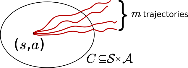 To simplify the notation, let $\pi = \pi_k$. A simple idea is rolling out with the policy $\pi$ from a fixed set $\mathcal{C}\subset \mathcal{S}\times \mathcal{A}$ to “approximately” measure the value of $\pi$ at the pairs in $\mathcal{C}$. For concreteness, let $(s,a)\in \mathcal{C}$. Rolling out with policy this pair means using the simulator to simulate what would happen if we used policy $\pi$ for a number of consecutive time steps when the initial state is $s$, the first action $a$, but for subsequent time steps the actions are chosen using policy $\pi$ for whatever states are encountered. If the simulation goes on for $H$ steps, this way we get \(m\) trajectories starting in \(z = (s, a)\). For $1\le j \le m$ let the trajectory obtained be \(\tau_\pi^{(j)}(s, a)\). Thus,
\(\begin{align*} \tau_\pi^{(j)}(s, a) = \left( S_0^{(j)}, A_0^{(j)}, S_1^{(j)}, A_1^{(j)}, \ldots, S_{H-1}^{(j)}, A_{H-1}^{(j)} \right)\, \end{align*}\),
where \(S_0^{(j)}=s\), \(A_0^{(j)}=a\), and for $1\le t \le H-1$, \(S_{t}^{(j)} \sim P_{A_t^{(j)}} ( S_{t-1}^{(j)} )\), and \(A_t^{(j)} \sim \pi ( \cdot | S_{t}^{(j)} )\). The figure on the right illustrates these trajectories.
Given these trajectories, the empirical mean of the discounted sum of rewards along these trajectories is used for approximating $q^\pi(z)$:
\[\begin{align} \hat R_m(z) = \frac{1}{m} \sum_{j=1}^m \sum_{t=0}^{H-1} \gamma^t r_{A_t^{(j)}}(S_t^{(j)}). \label{eq:petargetsbiased} \end{align}\]Under the usual condition that the rewards are in the $[0,1]$ interval, the expected value of $\hat{q}^\pi(z)$ is in the $\gamma^H/(1-\gamma)$ vicinity of the $q^\pi(z)$ and by averaging a large number of independent trajectories, we also achieve that the empirical means are tightly concentrated around their mean.
Using a randomization device, it is possible to remove the error (“bias”) introduced by truncating the trajectories at a fixed time. For this, just let $(H^{(j)})_{j}$ be independent geometrically distributed random variables with parameter $1-\gamma$, which are also independently chosen from the trajectories. By definition \(H^{(j)}\) is the number of $1-\gamma$-parameter Bernoulli trials needed to get one success. With the help of these variables, define now $\hat R_m(z)$ by
\[\begin{align} \hat R_m(z) = \frac{1}{m} \sum_{j=1}^m \sum_{t=0}^{H^{(j)}-1} r_{A_t^{(j)}}(S_t^{(j)})\,. \label{eq:petargetsunbiased} \end{align}\]Note that in the expression of \(\hat R_m(z)\) the discount factor is eliminated. To calculate \(\hat R_m(z)\) one can just perform a rollout with policy $\pi$ as before, just in each time step $t=0,1,\dots$, after obtaining $r_{A_t^{(j)}}(S_t^{(j)})$, draw a Bernoulli variable with parameter $(1-\gamma)$ to decide whether the rollout should continue.
To see why the above definition works, fix $j$ and note that by definition, for $h\ge 1$, \(\mathbb{P}(H^{(j)}=h) = \gamma^{h-1}(1-\gamma)\) and thus \(\mathbb{P}(H^{(j)}\ge t+1) = \gamma^t\). Therefore,
\[\begin{align*} \mathbb{E}[ \sum_{t=0}^{H^{(j)}-1} r_{A_t^{(j)}}(S_t^{(j)}) ] & = \sum_{t=0}^\infty \mathbb{E}[ \mathbb{I}\{ t \le H^{(j)}-1\} r_{A_t^{(j)}}(S_t^{(j)}) ] \\ & = \sum_{t=0}^\infty \mathbb{E}[ \mathbb{I}\{ t \le H^{(j)}-1\} ]\, \mathbb{E}[ r_{A_t^{(j)}}(S_t^{(j)}) ] \\ & = \sum_{t=0}^\infty \mathbb{P}( t+1 \le H^{(j)} )\, \mathbb{E}[ r_{A_t^{(j)}}(S_t^{(j)}) ] \\ & = \sum_{t=0}^\infty \gamma^t \mathbb{E}[ r_{A_t^{(j)}}(S_t^{(j)}) ] \\ & = q^\pi(z)\,. \end{align*}\]All in all, this means, that we expect that if we solve for the least-squares problem
\[\begin{align} \hat\theta = \arg\min_{\theta\in \mathbb{R}^d} \sum_{z\in \mathcal{C}} \left( \langle \theta,\varphi(z) \rangle - \hat R_m(z)\right)^2\,, \label{eq:lse} \end{align}\]we expect $\Phi \hat\theta$ to be a good approximation to $q^\pi$. Or at least, we can expect this hold at the points of $\mathcal{C}$, where we are taking our measurements. The question is what happens outside of $\mathcal{C}$: That is, what guarantees can we get for extrapolating to points of $\mathcal{Z}:= \mathcal{S}\times \mathcal{A}$. The first thing to observe that unless we are choosing $\mathcal{C}$ carefully, there is no guarantee about the extrapolation error will be kept under control. In fact, if the choice of $\mathcal{C}$ is so unfortunate that all the feature vectors for points in $\mathcal{C}$ are identical, the least-squares problem will have many solutions.
Our next lemma gives an explicit error bound on the extrapolation error. For the coming results we slightly generalize least-squares by introducing a weighting of the various errors in \(\eqref{eq:lse}\). For this, let $\varrho: \mathcal{C} \to (0,\infty)$ be a weighting function assigning a positive weight to the various error terms and let
\[\begin{align} \hat\theta = \arg\min_{\theta\in \mathbb{R}^d} \sum_{z\in \mathcal{C}} \varrho(z) \left( \langle \theta,\varphi(z) \rangle - \hat R_m(z)\right)^2 \label{eq:wlse} \end{align}\]be the minimizer of the resulting weighted squared-loss. A simple calculation gives that provided the (weighted) moment matrix
\[\begin{align} G_\varrho = \sum_{z\in \mathcal{C}} \varrho(z) \varphi(z) \varphi(z)^\top \label{eq:mommx} \end{align}\]is nonsingular, the solution to the above weighted least-squares problem is unique and is equal to
\[\hat{\theta} = G_\varrho^{-1} \sum_{z' \in C} \varrho(z') \hat R_m(z') \varphi(z')\,,\]From this expression we see that there is no loss of generality in assuming that the weights in the weighting function sum to one: \(\sum_{z\in \mathcal{C}} \varrho(z) = 1\). We will denote this by writing $\varrho \in \Delta_1(\mathcal{C})$ (here, $\Delta_1$ refers to the fact that we can see $\varrho$ as an element of a $|\mathcal{C}|-1$ simplex). To state the lemma recall the notation that for a positive definite, $d\times d$ matrix $Q$ and vector $x\in \mathbb{R}^d$,
\[\|x\|_Q^2 = x^\top Q x\,.\]Lemma (extrapolation error control in least-squares): Fix any \(\theta \in \mathbb{R}^d\), \(\varepsilon: \mathcal{Z} \rightarrow \mathbb{R}\), $\mathcal{C}\subset \mathcal{Z}$ and \(\varrho\in \Delta_1(\mathcal{C})\) such that the moment matrix $G_\varrho$ is nonsingular. Define
\[\begin{align*} \hat{\theta} = G_\varrho^{-1} \sum_{z' \in C} \varrho(z') \Big(\varphi(z')^\top \theta + \varepsilon(z') \Big) \varphi(z')\,. \end{align*}\]Then, for any \(z\in \mathcal{Z}\) we have
\[\left| \varphi(z)^\top \hat{\theta} - \varphi(z)^\top \theta \right| \leq \| \varphi(z) \|_{G_{\varrho}^{-1}}\, \max_{z' \in C} \left| \varepsilon(z') \right|\,.\]Before the proof note that what his lemma tells us is that as long as we guarantee that the moment matrix is full rank, the extrapolation errors relative to predicting with some $\theta\in \mathbb{R}^d$ can be controlled by controlling
- the value of \(g(\varrho):= \max_{z\in \mathcal{Z}} \| \varphi(z) \|_{G_{\varrho}^{-1}}\); and
- the maximum deviation of the targets used in the weighted least-squares problem and the predictions with $\theta$.
Proof: First, we relate $\hat\theta$ to $\theta$:
\[\begin{align*} \hat{\theta} &= G_\varrho^{-1} \sum_{z' \in C} \varrho(z') \Big(\varphi(z')^\top \theta + \varepsilon(z') \Big) \varphi(z') \\ &= G_\varrho^{-1} \left( \sum_{z' \in C} \varrho(z') \varphi(z') \varphi(z')^\top \right) \theta + G_\varrho^{-1} \sum_{z' \in C} \varrho(z') \varepsilon(z') \varphi(z') \\ &= \theta + G_\varrho^{-1} \sum_{z' \in C} \varrho(z') \varepsilon(z') \varphi(z'). \end{align*}\]Then for a fixed \(z \in \mathcal{Z}\),
\[\begin{align*} \left| \varphi(z)^\top \hat{\theta} - \varphi(z)^\top \theta \right| &= \left| \sum_{z' \in C} \varrho(z') \varepsilon(z') \varphi(z)^\top G_\varrho^{-1} \varphi(z') \right| \\ &\leq \sum_{z' \in C} \varrho(z') | \varepsilon(z') | \cdot | \varphi(z)^\top G_\varrho^{-1} \varphi(z') | \\ &\leq \Big( \max_{z' \in C} |\varepsilon(z')| \Big) \sum_{z' \in C} \varrho(z') | \varphi(z)^\top G_\varrho^{-1} \varphi(z') |\,. \end{align*}\]To get a sense of how to control the sum notice that if $\varphi(z)$ in the last sum was somehow replaced by $\varphi(z’)$, using the definition of $G_\varrho$ could greatly simplify the last expression. To get here, one may further notice that having the term in absolute value squared would help. Now, to get the squares, recall Jensen’s inequality, which states that for any convex function \(f\) and probability distribution \(\mu\), \(f \left(\int u \mu(du) \right) \leq \int f(u) \mu(du)\). Of course, this also works when $\mu$ is a finitely supported, which is the case here. Thus, applying Jensen’s inequality with \(f(x) = x^2\), we thus get
\[\begin{align*} \left(\sum_{z' \in C} \varrho(z') | \varphi(z)^\top G_\varrho^{-1} \varphi(z') |\right)^2 & \le \sum_{z' \in C} \varrho(z') | \varphi(z)^\top G_\varrho^{-1} \varphi(z') |^2 \\ &= \sum_{z' \in C} \varrho(z') \varphi(z)^\top G_\varrho^{-1} \varphi(z') \varphi(z')^\top G_\varrho^{-1} \varphi(z) \\ &= \varphi(z)^\top G_\varrho^{-1} \left( \sum_{z' \in C} \varrho(z') \varphi(z') \varphi(z')^\top \right) G_\varrho^{-1} \varphi(z) \\ &= \varphi(z)^\top G_\varrho^{-1} \varphi(z) = \|\varphi(z)\|_{G_\varrho^{-1}}^2 \end{align*}\]Plugging this back into the previous inequality gives the desired result. \(\qquad \blacksquare\)
It remains to be seen of whether \(g(\varrho)=\max_z \|\varphi(z)\|_{G_\varrho^{-1}}\) can be kept under control. This is the subject of a classic result of Kiefer and Wolfowitz:
Theorem (Kiefer-Wolfowitz): Let $\mathcal{Z}$ be finite. Let $\varphi: \mathcal{Z} \to \mathbb{R}^d$ be such that the underlying feature matrix $\Phi$ is rank $d$. There exists a set \(\mathcal{C} \subseteq \mathcal{Z}\) and a distribution \(\varrho: C \rightarrow [0, 1]\) over this set, i.e. \(\sum_{z' \in \mathcal{C}} \varrho(z') = 1\), such that
- \(\vert \mathcal{C} \vert \leq d(d+1)/2\);
- \(\sup_{z \in \mathcal{Z}} \|\varphi(z)\|_{G_\varrho^{-1}} \leq \sqrt{d}\);
- In the previous line, the inequality is achieved with equality and the value of $\sqrt{d}$ is best possible under all possible choices of $\mathcal{C}$ and $\rho$.
We will not give a proof of the theorem, but we give references at the end where the reader can look up the proof. When $\varphi$ is not full rank (i.e., $\Phi$ is not rank $d$), one may reduce the dimensionality (and the cardinality of $C$ reduces accordingly). The problem of choosing $\mathcal{C}$ and $\rho$ such that $g(\rho)$ is minimized is called the $G$-optimal design problem in statistics. This is a specific instance of optimal experimental design.
Combining the Kiefer-Wolfowitz theorem with the previous lemma shows that least-squares amplifies the “measurement errors” by at most a factor of \(\sqrt{d}\):
Corollary (extrapolation error control in least-squares via optimal design): Fix any $\varphi:\mathcal{Z} \to \mathbb{R}^d$ full rank. Then, there exists a set $\mathcal{C} \subset \mathcal{Z}$ with at most $d(d+1)/2$ elements and a weighting function \(\varrho\in \Delta_1(\mathcal{C})\) such that for any \(\theta \in \mathbb{R}^d\) and any \(\varepsilon: \mathcal{C} \rightarrow \mathbb{R}\),
\[\max_{z\in \mathcal{Z}}\left| \varphi(z)^\top \hat{\theta} - \varphi(z)^\top \theta \right| \leq \sqrt{d}\, \max_{z' \in C} \left| \varepsilon(z') \right|\,.\]where $\hat\theta$ is given by
\[\begin{align*} \hat{\theta} = G_\varrho^{-1} \sum_{z' \in C} \varrho(z') \Big(\varphi(z')^\top \theta + \varepsilon(z') \Big) \varphi(z')\,. \end{align*}\]Importantly, note that $\mathcal{C}$ and $\varrho$ are chosen independently of $\theta$ and $\epsilon$, that is, they are independent of the target. This suggests that in approximate policy evaluation, one should choose $(\mathcal{C},\rho)$ as in the Kiefer-Wolfowitz theorem and use the $\rho$ weighted moment matrix. This leads to \(\begin{align} \hat{\theta} = G_\varrho^{-1} \sum_{z' \in C} \varrho(z') \hat R_m(z') \varphi(z')\,. \label{eq:lspeg} \end{align}\) where $\hat R_m(z)$ is defined by Eq. \(\eqref{eq:petargetsbiased}\) and $G_\varrho$ is defined by Eq. \(\eqref{eq:mommx}\). We call this procedure least-square policy evaluation based on rollouts from $G$-optimal design points, or LSPE-$G$, for short. Note that we stick to the truncated rollouts, because this allows a simpler probabilistic analysis. That this properly controls the extrapolation error is as attested by the next result:
Lemma (LSPE-$G$ extrapolation error control): Fix any full-rank feature-map $\varphi:\mathcal{Z} \to \mathbb{R}^d$ and take the set $\mathcal{C} \subset \mathcal{Z}$ and the weighting function \(\varrho\in \Delta_1(\mathcal{C})\) as in the Kiefer-Wolfowitz theorem. Fix an arbitrary policy $\pi$ and let $\theta$ and $\varepsilon_\pi$ such that $q^\pi = \Phi \theta + \varepsilon_\pi$ and assume that immediate rewards belong to the interval $[0,1]$. Let $\hat{\theta}$ be as in Eq. \eqref{eq:lspeg}. Then, for any $0\le \delta \le 1$, with probability $1-\delta$,
\[\begin{align} \left\| q^\pi - \Phi \hat{\theta} \right\|_\infty &\leq \|\varepsilon_\pi\|_\infty (1 + \sqrt{d}) + \sqrt{d} \left(\frac{\gamma^H}{1 - \gamma} + \frac{1}{1 - \gamma} \sqrt{\frac{\log(2 \vert C \vert / \delta)}{2m}}\right). \label{eq:lspeee} \end{align}\]Notice that that from the Kiefer-Wolfowitz theorem, \(\vert C \vert = O(d^2)\) and therefore nothing in the above expression depends on the size of the state space. Now, say we want to make the above error bound at most \(\|\varepsilon_\pi\|_\infty (1 + \sqrt{d}) + 2\varepsilon\) with some value of $\varepsilon>0$. From the above we see that it suffices to choose $H$ and $m$ so that
\[\begin{align*} \frac{\gamma^H}{1 - \gamma} \leq \varepsilon/\sqrt{d} \qquad \text{and} \qquad \frac{1}{1 - \gamma} \sqrt{\frac{\log(2 \vert C \vert / \delta)}{2m}} \leq \varepsilon/\sqrt{d}. \end{align*}\]This, together with \(\vert\mathcal{C}\vert\le d(d+1)/2\) gives
\[\begin{align*} H \geq H_{\gamma, \varepsilon/\sqrt{d}} \qquad \text{and} \qquad m \geq \frac{d}{(1 - \gamma)^2 \varepsilon^2} \, \log \frac{d(d+1)}{\delta}\,. \end{align*}\]Proof: In a nutshell, we use the previous corollary, together with Hoeffding’s inequality and using that $|q^\pi-T_\pi^H \boldsymbol{0}|_\infty \le \gamma^H/(1-\gamma)$, which follows since the rewards are bounded in $[0,1]$.
Click here for the full proof.
Fix $z\in \mathcal{C}$. Let us write $\hat{R}_m(z) = q^\pi(z) + \hat{R}_m(z) - q^\pi(z) = \varphi(z)^\top \theta + \varepsilon(z)$ where we define $\varepsilon(z) = \hat{R}_m(z) - q^\pi(z) + \varepsilon_\pi(z)$. Then $$ \hat{\theta} = G_\varrho^{-1} \sum_{z' \in C} \varrho(z') \Big( \varphi(z')^\top \theta + \varepsilon(z') \Big) \varphi(z'). $$ Now we will bound the difference between our action-value function estimate and the true action-value function: $$ \begin{align} \| q^\pi - \Phi \hat\theta \|_\infty & \le \| \Phi \theta - \Phi \hat\theta\|_\infty + \| \varepsilon_\pi \|_\infty \le \sqrt{d}\, \max_{z\in \mathcal{C}} |\varepsilon(z)|\, + \| \varepsilon_\pi \|_\infty \label{eq:bound_q_values} \end{align} $$ where the last line follows from the Corollary above. For bounding the first term above, first note that $\mathbb{E} \left[ \hat{R}_m(z) \right] = (T_\pi^H \mathbf{0})(z)$. Then, $$ \begin{align*} \varepsilon(z) &= \hat{R}_m(z) - q^\pi(z) + \varepsilon_\pi(z) \nonumber \\ &= \underbrace{\hat{R}_m(z) - (T_\pi^H \mathbf{0})(z)}_{\text{sampling error}} + \underbrace{(T_\pi^H \mathbf{0})(z) - q^\pi(z)}_{\text{truncation error}} + \underbrace{\varepsilon_\pi(z)}_{\text{fn. approx. error}}. \end{align*} $$ Since the rewards are assumed to belong to the unit interval, the truncation error is at most $\frac{\gamma^H}{1 - \gamma}$. Concerning the sampling error (first term), Hoeffding's inequality gives that for any given $z\in \mathcal{C}$, $ \left \vert \hat{R}_m(z) - (T_\pi^H \mathbf{0})(z) \right \vert \leq \frac{1}{1 - \gamma} \sqrt{\frac{\log(2 / \delta)}{2m}}$ with at least $1 - \delta$ probability. Applying a union bound, we get that with probability at least $1 - \delta$, for all $z \in \mathcal{C}$, $ \left \vert \hat{R}_m(z) - (T_\pi^H \mathbf{0})(z) \right \vert \leq \frac{1}{1 - \gamma} \sqrt{\frac{\log(2 \vert C \vert / \delta)}{2m}}$. Putting things together, we get that with probability at least $1 - \delta$, $$ \begin{equation} \max_{z \in \mathcal{C}} | \varepsilon(z) | \leq \frac{\gamma^H}{1 - \gamma} + \frac{1}{1 - \gamma} \sqrt{\frac{\log(2 \vert C \vert / \delta)}{2m}} + \|\varepsilon_\pi\|_\infty\,. \label{eq:bound_varepsilon_z} \end{equation} $$ Plugging this into Eq. \eqref{eq:bound_q_values} and algebra gives the desired result.\(\blacksquare\)
In summary, what we have shown so far is that if the features can approximate well the action-value function of a policy, then there is a simple procedure (Monte-Carlo rollouts and least-squares estimation based on an optimal experimental design) to produce an reliable estimate of the action-value function of the policy. The question remains whether if we use these estimates in policy iteration, the whole procedure will still give good policies after a sufficiently large number of iterations.
Progress Lemma with Approximation Errors
Here we give a refinement of the geometric progress lemma of policy iteration that allows for “approximate” policy improvement steps. This previous lemma stated that the value function of the improved policy $\pi’$ is at least as large as the Bellman operator applied to the value function of the policy $\pi$ to be improved. Our new lemma is as follows:
Lemma (Geometric progress lemma with approximate policy improvement): Consider a memoryless policy \(\pi\) and its corresponding value function \(v^\pi\). Let \(\pi'\) be any policy and define $\varepsilon:\mathcal{S} \to \mathbb{R}$ via
\[T v^\pi = T_{\pi'} v^{\pi} + \varepsilon\,.\]Then,
\[\|v^* - v^{\pi'}\|_\infty \leq \gamma \|v^* - v^{\pi}\|_\infty + \frac{1}{1 - \gamma} \, \|\varepsilon\|_\infty.\]Proof: First note that for the optimal policy \(\pi^*\), \(T_{\pi^*} v^* = v^*\). We have
\[\begin{align} v^* - v^{\pi'} & = T_{\pi^*}v^* - T_{\pi^*} v^{\pi} + \overbrace{T_{\pi^*} v^\pi}^{\le T v^\pi} - T_{\pi'} v^\pi + T_{\pi'} v^{\pi} - T_{\pi'} v^{\pi'} \nonumber \\ &\le \gamma P_{\pi^*} (v^*-v^\pi) + \varepsilon + \gamma P_{\pi'} (v^\pi-v^{\pi'})\,. \label{eq:vstar_vpiprime} \end{align}\]Using the value difference identity and that $v_\pi =T_\pi v^\pi\le T v^\pi$, we calculate
\[\begin{align*} v^\pi - v^{\pi'} = (I-\gamma P_{\pi'})^{-1} [ v^\pi - T_{\pi'}v^\pi] \le (I-\gamma P_{\pi'})^{-1} [ T v^\pi - (T v^\pi -\varepsilon) ] = (I-\gamma P_{\pi'})^{-1} \varepsilon\,, \end{align*}\]where the inequality follows because $(I-\gamma P_{\pi’})^{-1}= \sum_{k\ge 0} (\gamma P_{\pi’})^k$, the sum of positive linear operators, is a positive linear operator itself and hence is also monotone. Plugging the inequality obtained into \eqref{eq:vstar_vpiprime} gives
\[\begin{align*} v^* - v^{\pi'} \le \gamma P_{\pi^*} (v^*-v^\pi) + (I-\gamma P_{\pi'})^{-1} \varepsilon. \end{align*}\]Taking the maximum norm of both sides and using the triangle inequality and that \(\| (I-\gamma P_{\pi'})^{-1} \|_\infty \le 1/(1-\gamma)\) gives the desired result. \(\qquad \blacksquare\)
Approximate Policy Iteration
Notice that the progress lemma makes no assumptions about the origin of the errors. This motivates considering a generic version of approximate policy iteration where for $k\ge 1$ in the $k$th update set, the new policy $\pi_k$ is approximately greedy with respect to $v^{\pi_k}$ in that sense that
\[\begin{align} T v^{\pi_k} = T_{\pi_{k+1}} v^{\pi_k} + \varepsilon_k\,. \label{eq:apidef} \end{align}\]The progress lemma implies that the resulting sequence of policies will have value functions that converge to a neighborhood of $v^*$ where the size of the neighborhood is governed by the magnitude of the error terms \((\varepsilon_k)_k\).
Theorem (Approximate Policy Iteration): Let \((\pi_k)_{k\ge 0}\), \((\varepsilon_k)_k\) be such that \eqref{eq:apidef} holds for all \(k\ge 0\). Then, for any \(k\ge 1\),
\[\begin{align} \|v^* - v^{\pi_k}\|_\infty \leq \frac{\gamma^k}{1-\gamma} + \frac{1}{(1-\gamma)^2} \max_{0\le s \le k-1} \|\varepsilon_{s}\|_\infty\,. \label{eq:apieb} \end{align}\]Proof: Left as an exercise. \(\qquad \blacksquare\)
Consider now a version of approximate policy iteration where the sequence of policies \((\pi_k)_{k\ge 0}\) is defined as follows:
\[\begin{align} q_k = q^{\pi_k} + \varepsilon_k', \qquad M_{\pi_{k+1}} q_k = M q_k\,, \quad k=0,1,\dots\,. \label{eq:apiavf} \end{align}\]That is, for each \(k=0,1,\dots\), \(\pi_k\) is greedy with respect to \(q_{k-1}\).
Corollary (Approximate Policy Iteration with Approximate Action-value Functions): The sequence defined in \eqref{eq:apiavf} is such that
\[\| v^* - v^{\pi_k} \|_\infty \leq \frac{\gamma^k}{1-\gamma} + \frac{2}{(1-\gamma)^2} \max_{0\le s \le k-1} \|\varepsilon_{s}'\|_\infty\,.\]Proof: To simplify the notation consider policies \(\pi,\pi'\) and functions \(q,\varepsilon'\) over the state-action space such that \(M_{\pi'} q = M q\) and \(q=q^\pi+\varepsilon'\). We have
\[\begin{align*} T v^\pi & \ge T_{\pi'} v^\pi = M_{\pi'} (r+\gamma P v^\pi) = M_{\pi'} q^\pi = M_{\pi'} q - M_{\pi} \varepsilon' = M q - M_\pi \varepsilon'\\ & \ge M (q^\pi - \|\varepsilon'\|_\infty \boldsymbol{1}) - M_\pi \varepsilon' \ge M q^\pi - 2 \|\varepsilon'\|_\infty \boldsymbol{1} = T v^\pi - 2 \|\varepsilon'\|_\infty \boldsymbol{1}\,, \end{align*}\]where we used that \(M_\pi\) is linear, monotone, and that $M$ is monotone, and both are nonexpansions in the maximum norm.
Hence, if $\varepsilon_k$ is defined by \eqref{eq:apidef} then \(\|\varepsilon_k\|_\infty \le 2 \|\varepsilon_k'\|_\infty\) and the result follows from the previous theorem. \(\qquad \blacksquare\)
Global planning with least-squares policy iteration
Putting things together gives the following planning method:
- Given the feature map $\varphi$, find \(\mathcal{C}\) and \(\rho\) as in the Kiefer-Wolfowitz theorem
- Let \(\theta_{-1}=0\)
- For \(k=0,1,2,\dots,K-1\) do
- \(\qquad\) Roll out with policy \(\pi:=\pi_k\) for $H$ steps to get the targets \(\hat R_m(z)\) where \(z\in \mathcal{C}\)
\(\qquad\) and \(\pi_k(s) = \arg\max_a \langle \theta_{k-1}, \varphi(s,a) \rangle\) - \(\qquad\) Solve the weighted least-squares problem given by Eq. \(\eqref{eq:wlse}\) to get \(\theta_k\).
- Return \(\theta_{K-1}\)
We call this method least-squares policy iteration (LSPI) for obvious reasons. Note that this is a global planning method: The method makes no use of an input state and the parameter vector returned can be used to get the policy $\pi_{K}$ (as in the method above).
Theorem (LSPI performance): Fix an arbitrary full rank feature-map $\varphi: \mathcal{S}\times \mathcal{A} \to \mathbb{R}^d$ and let $K,m,H\ge 1$. Assume that B2\(_{\varepsilon}\) holds. Then, for any $0\le \zeta \le 1$, with probability at least $1-\zeta$, the policy $\pi_{K}$ which is greedy with respect to $\Phi \theta_{K-1}$ is $\delta$-suboptimal with
\[\begin{align*} \delta \le \underbrace{\frac{2(1 + \sqrt{d})}{(1-\gamma)^2}\, \varepsilon}_{\text{approx. error}} + \underbrace{\frac{\gamma^{K-1}}{1-\gamma}}_{\text{iter. error}} + \underbrace{\frac{2\sqrt{d}}{(1-\gamma)^3} \left(\gamma^H + \sqrt{\frac{\log( d(d+1)K / \zeta)}{2m}}\right)}_{\text{pol.eval. error}} \,. \end{align*}\]In particular, for any $\varepsilon’>0$, choosing $K,H,m$ so that
\[\begin{align*} K & \ge H_{\gamma,\gamma\varepsilon'/2} \\ H & \ge H_{\gamma,(1-\gamma)^2\varepsilon'/(8\sqrt{d})} \qquad \text{and} \\ m & \ge \frac{32 d}{(1-\gamma)^6 (\varepsilon')^2} \log( (d+1)^2 K /\zeta ) \end{align*}\]policy $\pi_K$ is $\delta$-optimal with
\[\begin{align*} \delta \le \frac{2(1 + \sqrt{d})}{(1-\gamma)^2}\, \varepsilon + \varepsilon'\,, \end{align*}\]while the total computation cost is $\text{poly}(\frac{1}{1-\gamma},d,\mathrm{A},\frac{1}{\varepsilon’},\log(1/\zeta))$.
Thus, with a polynomial cost, LSPI with the specific configuration at the cost of polynomial computation cost, but importantly, with a cost that is independent of the size of the state space, can result in a good policy as long as $\varepsilon$, the worst-case error of approximating action-value functions of policies using the features provided, is sufficiently small.
Proof: Note that B2\(_\varepsilon\) and that $\Phi$ is full rank implies that for any memoryless policy $\pi$ there exists a parameter vector $\theta\in \mathbb{R}^d$ such that \(\| \Phi \theta - q^\pi \|_\infty \le \varepsilon\) (cf. Part 2 of Question 3 of Assignment 2). Hence, we can use the “LSPE extrapolation error bound” (cf. \(\eqref{eq:lspeee}\)). By this result, a union bound and of course by B2$_\varepsilon$, we get that for any $0\le \zeta \le 1$, with probability at least $1-\zeta$, for any $0 \le k \le K-1$,
\[\begin{align*} \| q^{\pi_k} - \Phi \theta_k \|_\infty &\leq \varepsilon (1 + \sqrt{d}) + \sqrt{d} \left(\frac{\gamma^H}{1 - \gamma} + \frac{1}{1 - \gamma} \sqrt{\frac{\log( d(d+1)K / \zeta)}{2m}}\right)\,, \end{align*}\]where we also used that \(\vert \mathcal{C} \vert \le d(d+1)\). Call the quantity on the right-hand side in the above inequality $\kappa$.
Take the event when the above inequalities hold and for now assume this event holds. By the previous theorem, $\pi_K$ is $\delta$-optimal with
\[\delta \le \frac{\gamma^{K-1}}{1-\gamma} + \frac{2}{(1-\gamma)^2} \kappa \,.\]To obtain the second part of the result, we split $\varepsilon’$ into two equal parts: $K$ is set to force the iteration error to be at most $\varepsilon’/2$, while $H$ and $m$ are chosen to force the policy evaluation error to be at most $\varepsilon’/2$. Here, to choose $H$ and $M$, $\varepsilon’/2$ is again split into two equal parts. The details of this calculation are left to the reader. \(\qquad \blacksquare\)
Notes
Approximate Dynamic Programming (ADP)
Value iteration and policy iteration are specific instances of dynamic programming methods. In general, dynamic programming refers to methods that use value functions to calculate good policies. In approximate dynamic programming the methods are modified by introducing “errors” when calculating the values. The idea is that the origin of the errors does not matter (e.g., whether they come due to imperfect function approximation, linear, or nonlinear, or due to the sampling): The analysis is done in a general form. While here we met approximate policy iteration, one can also use the same ideas as shown here to study an approximate version of value iteration. A homework in problem set 2 asks you to study this method, which is usualy called approximate value iteration. In an earlier homework you were asked to study how linear programming can also be used to compute optimal value functions. Adding approximations we then get approximate linear programming.
What function approximation technique to use?
We note in passing that fans of neural networks should like that the general, ADP-style results, like the theorem in the middle of this lecture, can be also applied to the case when neural networks are used as the function approximation technique. However, one main lesson of the lecture is that to control extrapolation errors, one should be quite careful in how the training data is chosen. For linear prediction and least-squares fitting, optimal design gives a complete answer, but the analog questions are completely open in the case of nonlinear function approximation, such as neural networks. There is also a sizable literature that connects nonparametric techniques (an analysis friendly relative of neural networks) to ADP methods.
Concentrability coefficients and all that jazz
The idea of introducing approximate calculations has been introduced at the same time people got interested in Markov Decision Processes in the 1960s. Hence, the literature is quite enormous. However, the approach taken here which asks for error bounds where the algorithmic (not approximation-) error is uniformly controlled regardless of the MDP is quite recent and where the term that involves the approximation error is also uniformly bounded (for a fixed dimension and discount factor).
Earlier literature often presented bounds where the magnification factor of the approximation and the algorithmic error involved terms which depended on the MDP. Often these came in the form of “concentrability coefficients” (and yours truly was quite busy with working on these results a while ago). The main conclusion of this earlier analysis is that more stochasticity in the transitions means less control, less concentrability, which is advantageous for the ADP algorithms. While this makes sense and this indicates that these earlier results are complementary to the results presented here, the issue is that these results are quite pessimistic for example when the MDP is deterministic (as in this case the concentrability coefficients can be as large as the size of the state space).
While here we emphasized the importance of using a good design to control the extrapolation errors, in these earlier results, no optimal design was used. The upshot is that this saves the effort of coming up with a good design, but the obvious downside is that the extrapolation error may become uncontrolled. In the batch setting (which we will come back to later), of course, there is no way to control the sample collection, and this is in fact the setting where this earlier analysis was done.
The strength of hints
A critical assumption in the analysis of API was that the approximation error is controlled uniformly for all policies. This feels limiting. Yet, there are some interesting sufficient conditions when this assumption is clearly satisfied. In general, these require that the transition dynamics and the reward are both “compressible”. For example, if the MDP is such that $r$, the immediate reward as a function of the state-action pairs satisfies \(r = \Phi \theta_r\) and the transition matrix, \(P\in [0,1]^{\mathrm{S}\mathrm{A} \times \mathrm{S}}\) satisfies \(P = \Phi H\) with some matrix \(H\in \mathbb{R}^{d\times \mathrm{S}}\), then for any policy policy \(\pi\), \(T_\pi q = r+ \gamma P M_\pi q\) has a range which is a subset of \(\text{span}(\Phi)=\mathcal{F}_{\varphi}\). Since \(q^\pi\) is the fixed-point of \(T_\pi\), i.e., \(q^\pi = T_\pi q^\pi\), it follows that \(q^\pi\) is also necessarily in the range space of \(T_\pi\). As such, \(q^\pi \in \mathcal{F}_{\varphi}\) and \(\varepsilon_{\text{apx}}=0\). MDPs that satisfy the above two constraints are called linear in \(\Phi\) (or sometimes, just “linear MDPs”). Exact linearity can be relaxed: If \(r = \Phi \theta_r + \varepsilon_r\) and \(P = \Phi H +E\), then for any policy \(\pi\), \(q^\pi\in_{\varepsilon} \mathcal{F}_{\varphi}\) with \(\varepsilon \le \|\varepsilon_r\|_\infty+\frac{\gamma}{1-\gamma}\|E\|_\infty\). Nevertheless, later we will investigate whether this assumption can be relaxed.
The tightness of the bounds
It is not known whether the bound presented in the final result is tight. In fact, the dependence of $m$ on the $1/(1-\gamma)$ is almost certainly not tight; in similar scenarios it has been shown in the past that replacing Hoeffding’s inequality with Bernstein’s inequality allows the reduction of this factor. It is more interesting whether the amplification factor of the approximation error, $\sqrt{d}/(1-\gamma)^2$, is best possible. In the next lecture we will show that the $\sqrt{d}$ approximation error amplification factor cannot be removed while keeping the runtime under control. In a later lecture, we will show that the dependence on $1/(1-\gamma)$ cannot be improved either – at least for this algorithm. However, we will see that if the main concern is the amplification of the approximation error, while keeping the runtime polynomial (perhaps with a higher order though) then under B2\(_{\varepsilon}\) better algorithms exist.
The cost of optimal experimental design
The careful reader would not miss that to run the proposed method one needs to find the set $\mathcal{C}$ and the weighting function $\rho$. The first observation here is that it is not crucial to find the best possible $(\mathcal{C},\rho)$ pair. The Kiefer-Wolfowitz theorem showed that with this best possible choice, $g(\rho) = \sqrt{d}$. However, if one finds a pair such that $g(\rho)=2\sqrt{d}$, the price of this is that wherever $\sqrt{d}$ appears in the final performance bound, a submultiplicative factor of $2$ will also need to be introduced. This should be acceptable. In relation to this note that by relaxing this optimality requirement, the cardinality of $\mathcal{C}$ can be reduced. For example, by introducing the factor of $2$ as suggested above allows one to reduce the cardinlity to $O(d \log \log d)$; which may actually be a good tradeoff as this can save much on the runtime.
However, the question still remains of who computes these (approximately) optimal designs and at what cost. While this calculation only needs to be done once and is independent of the MDP (just depends on the feature map), the value of these methods remains unclear because of this compute cost. General methods to compute approximately optimal designs needed here are known, but their runtime for our case will be proportional to the number of state-action pairs. In the very rare cases when simulating transitions is very costly but the number of state-action pairs is not too high, this may be a viable option. However, these cases are rare. For special choices of the feature-map, optimal designs may be known. However, this reduces the general applicability of the method presented here. Thus, a major question is whether the optimal experimental design can be avoided. What is known is that for linear prediction with least-squares, clearly, they cannot be avoided. One suspects that this is true more generally.
Can optimal designs be avoided while keeping the results essentially unchanged? Of particular interest would be if the feature-map would also be only “locally explored” as the planner interacts with the simulator. Altogether, one suspects that two factors contributed here for the appearance of optimal experimental design: One factor is that the planner is global: It comes up with a parameter vector that leads to a policy that can be used regardless of the state. The other (perhaps) factor is that the approach was based on simple “patching up” a dynamic programming algorithm with a function approximator. While this is a common approach, controlling the extrapolation errors in this approach is critical and is likely only possible with something like an optimal experimental design. As we shall see soon, there are indeed approaches that avoid the optimal experimental design step and which are based on online planning and they also deviate from the ADP approach.
Policy evaluation alternatives
The policy evaluation method presented here feels unsophisticated. It uses simple Monte-Carlo rollouts, with truncation, averaging and least-squares regression. The reinforcement learning literature offers many alternatives, such as the “temporal difference” learning type methods that are based on solving the fixed point equation $q^\pi = T_\pi q^\pi$. One can indeed try to use this equation to avoid the crude Monte-Carlo approach presented here, in the hope of reducing the variance (which is currently rather crudely upper bounded using the $1/(1-\gamma)$ term in the Hoeffding bound). Rewriting the fixed point as $(I-\gamma P_\pi) q^\pi = r$, and then plugging in $q^\phi = \Phi \theta + \varepsilon$, we see that the trouble is that to control the extrapolation errors, the optimal design must likely depend on the policy to be evaluated (because of the appearance of $(I-\gamma P_\pi)\Phi$).
Alternative error control: Bellman residuals
Let \((\pi_k)_{k\ge 0}\) and \((q_k,\varepsilon_k)_{k\ge 0}\) be so that
\[\varepsilon_k = q_k - T_{\pi_k} q_k\]Here, \(\varepsilon_k\) is called the “Bellman residual” of \(q_k\). The policy evaluation alternatives above aim at controlling these residuals. The reader is invited to derive the analogue of the “approximate policy iteration” error bound in \eqref{eq:apieb} for this scenario.
The role of $\rho$ in the Kiefer-Wolfowitz result
One may wonder about how critical is the presence of $\rho$ in the results presented. For this, we can say that it is not critical. Unweighted least-squares does not perform much worse.
Least-squares error bound
The error bound presented for least-squares does not use the full power of randomness. When part of the errors $\varepsilon(z)$ with $z\in \mathcal{C}$ are random, some helpful averaging effects can appear, which we ignored for now, but which could be used in a more refined analysis.
Optimal experimental design – a field on its own
Optimal exoerimental design is a subfield of statistics. The design considered here is just one possibility. In fact, this design which is called G-optimal design (G stands, uninspiringly, for the word “general”). The Kiefer-Wolfowitz theorem actually also states that this is equivalent to the D-optimal designs.
Lack of convergence
The results presented show convergence to a ball around the optimal target. Some people think this is a major concern. While having a convergent method may look more appealing, as long as one controls the size of the ball, I will not be too concerned.
Approximate value iteration (AVI)
Similarly to what is done here, one can introduce an approximate version of value-iteration. This is the subject of Question 3 of homework 2. While the conditions are different, the qualitative behavior of AVI is similar to that of approximate policy iteration.
In particular, as for approximate policy iteration, there are two steps to this proof: One is to show that the residuals $\varepsilon_k = q_k - T q_{k-1}$ can be controlled and the second is that if they are controlled then the policy that is greedy with respect to (say) $q_K$ is $\delta$-optimal with $\delta$ controlled by \(\varepsilon_{1:K}:=\max_{1\le k \le K} \| \varepsilon_k \|_\infty\). For this second part, we have the following bound:
\[\begin{align} \delta \le 2 H^2 (\gamma^K + \varepsilon_{1:K})\,. \label{eq:lsvibound} \end{align}\]where $H=1/(1-\gamma)$. The procedure that uses least-squares fitting to get the iterates $(q_k)_k$ is known under various names, such as least-squares value iteration (LSVI), fitted Q-iteration (FQI), least-squares Q iteration (LSQI). This proliferation of abbreviations and names is unfortunate, but there is not much that can be done at this stage. To add insult to injury, when neural networks are used to represent the iterates and an incremental stochastic gradient descent algorithm is used for “fitting” the weights of these networks by resampling old data from a “replay buffer”, the resulting procedure is coined “Deep Q-Networks” (training), or DQN for short.
Bounds on the parameter vector
The Kiefer-Wolfowitz theorem implies the following:
Proposition: Let $\phi:\mathcal{Z}\to\mathbb{R}^d$ and $\theta\in \mathbb{R}^d$ be such that $\sup_{z\in \mathcal{Z}}|\langle \phi(z),\theta \rangle|\le 1$ and \(\sup_{z\in \mathcal{Z}} \|\phi(z)\|_2 <+\infty\). Then, there exist a matrix $S\in \mathbb{R}^{d\times d}$ such that for $\tilde \phi$
\[\begin{align*} \tilde\phi(z) & = S\phi(z)\,, \qquad z\in \mathcal{Z} \end{align*}\]there exists \(\tilde \theta\in \mathbb{R}^d\) such that the following hold:
- \(\langle \phi(z),\theta \rangle = \langle \tilde \phi(z),\tilde \theta \rangle\), \(z\in \mathcal{Z}\);
- \(\sup_{z\in \mathcal{Z}} \| \tilde \phi(z) \|_2 \le 1\);
- \(\|\tilde \theta \|_2 \le \sqrt{d}\).
Proof: Let $\rho:\mathcal{Z} \to [0,1]$ be the $G$-optimal design whose existence is guaranteed by the Kiefer-Wolfowitz theorem. Let \(M = \sum_{z\in \mathrm{supp}(\rho)} \rho(z) \phi(z)\phi(z)^\top\) be the underlying moment matrix. Then, by the definition of $\rho$, \(\sup_{z\in \mathcal{Z}}\|\phi(z)\|_{M^{-1}}^2 \le d\).
Define \(S= (dM)^{-1/2}\) and \(\tilde \theta = S^{-1} \theta\). The first property is clearly satisfied. As to the second property,
\[\|\tilde \phi(z)\|_2^2 = \| (dM)^{-1/2}\phi(z)\|_2^2 = \phi(z)^\top (dM)^{-1} \phi(z) \le 1\,.\]Finally, for the third property,
\[\| \tilde \theta \|_2^2 = d \theta^\top \left( \sum_{z\in \mathrm{supp}(\rho)} \rho(z) \phi(z) \phi(z)^\top \right) \theta = d \sum_{z\in \mathrm{supp}(\rho)} \rho(z) \underbrace{(\theta^\top \phi(z))^2}_{\le 1} \le d\,,\]finishing the proof. \(\qquad \blacksquare\)
Thus, if one has access to the full feature-map then knowing that a function realized is bounded, one may as well assume that the feature map is bounded and the parameter vector is bounded just by $\sqrt{d}$.
Regularized least-squares
The linear least-squares predictor given by a feature-map $\phi$ and data $(z_1,y_1),\dots,(z_n,y_n)$ predicts a response at $z$ via $\langle \phi(z),\hat\theta \rangle$ where
\[\begin{align} \hat\theta = G^{-1}\sum_{i=1}^n \phi_i y_i\,, \label{eq:ridgesol} \end{align}\]with
\[G = \sum_{i=1}^n \phi_i \phi_i^\top\,.\]Here, by abusing notation for the sake of minimizing clutter, we use $\phi_i=\phi(z_i)$, $i=1,\dots,n$. The problem is that $G$ may not be invertible (i.e., $\hat \theta$ may not be defined as written above). “By continuity”, it is nearly equally problematic when $G$ is ill-conditioned (i.e., its minimum eigenvalue is “much smaller” than its maximum eigenvalue). In fact, this leads to poor “generalization”. One remedy, often used, is to modify $G$ by shifting it with a small constant multiple of the identity matrix:
\[G = \lambda I + \sum_{i=1}^n \phi_i \phi_i^\top\,.\]Here, $\lambda>0$ is a tuning parameter, whose value is often chosen based on cross-validation or with a similar process. The modification guarantees that $G$ is invertible and it overall improves the quality of predictions, especially when $\lambda$ is tuned base on data.
Above, the choice of the identity matrix, while is common in the literature, is completely arbitrary. In particular, invertibility will be guaranteed if $I$ is replaced with any other positive definite matrix $P$. In fact, the matrix one should use here should be one that makes $|\theta|_P^2$ small (while, say, keeping the minimum eigenvalue of $P$ at constant). That this is the choice that makes sense can be argued for by noting that with
\[G = \lambda P + \sum_{i=1}^n \phi_i \phi_i^\top\,.\]the $\hat\theta$ vector defined in \eqref{eq:ridgesol} is the minimizer of
\[L_n(\theta) = \sum_{i=1}^n ( \langle \phi_i,\theta \rangle - y_i)^2 \,\,+ \lambda \| \theta\|_P^2\,,\]and thus, the extra penalty has the least impact for the choice of $P$ that makes the norm of $\theta$ the smallest. If we only know that $\sup_{z} |\langle \phi(z),\theta \rangle|\le 1$, by our previous note, a good choice is $P=d M$, where \(M = \sum_{z\in \mathrm{supp}(\rho)} \rho(z) \phi(z)\phi(z)^\top\) where \(\rho\) is a $G$-optimal design. Indeed, with this choice, \(\|\theta\|_P^2 = d \|\theta \|_M^2 \le d\). Note also that if we apply the feature-standardization transformation of the previous note, we have
\[(dM)^{-1/2} (\sum_i \phi_i \phi_i^\top + \lambda d M ) (dM)^{-1/2} = \sum_i \tilde \phi_i \tilde \phi_i^\top + \lambda I\,,\]showing that the choice of using the identity matrix is justified when the features are standardized as in the proposition of the previous note.
References
We will only scratch the surface now; expect more references to be added later.
The bulk of this lecture is based on
- Tor Lattimore, Csaba Szepesvári, and Gellért Weisz. 2020. “Learning with Good Feature Representations in Bandits and in RL with a Generative Model.” ICML and arXiv:1911.07676,
who introduced the idea of using \(G\)-optimal designs for controlling the extrapolation errors. A very early reference on error bounds in “approximate dynamic programming” is the following:
- Whitt, Ward. 1979. “Approximations of Dynamic Programs, II.” Mathematics of Operations Research 4 (2): 179–85.
The analysis of the generic form of approximate policy iteration is a refinement of Proposition 6.2 from the book of Bertsekas and Tsitsiklis:
- Dimitri P. Bertsekas and John N. Tsitsiklis. Neuro-Dynamic Programming. Athena Scientific, Belmont, Massachusetts, 1996.
However, there are some differences between the “API” theorem presented here and Proposition 6.2. In particular, the theorem presented here appears to capture all sources of errors in a general way, while Proposition 6.2 is concerned with value function approximation errors and errors introduced in the “greedification step”. The form adopted here appears, for example, in Theorem 1 of a technical report of Scherrer, who also gives earlier references:
- Scherrer, Bruno. 2013. “On the Performance Bounds of Some Policy Search Dynamic Programming Algorithms.” arxiv.
The earliest of these references is perhaps
- Munos, R. 2003. “Error Bounds for Approximate Policy Iteration.” ICML.
Least-squares policy iteration appears in
- Lagoudakis, M. G. and Parr, R. Least-squares policy iteration. The Journal of Machine Learning Re-search, 4:1107–1149, 2003.
The particular form presented in this work though uses value function approximation based on minimizing the Bellman residuals (using the so-called LSTD method).
Two books that advocate the ADP approach:
- Powell, Warren B. 2011. Approximate Dynamic Programming. Solving the Curses of Dimensionality. Hoboken, NJ, USA: John Wiley & Sons, Inc.
- Lewis, Frank L., and Derong Liu. 2013. Reinforcement Learning and Approximate Dynamic Programming for Feedback Control. Hoboken, NJ, USA: John Wiley & Sons, Inc.
And a chapter:
- Bertsekas, Dimitri P. 2009. “Chapter 6: Approximate Dynamic Programming,” January, 1–118.
A paper that is concerned with API and least-squares methods, but uses concentrability is:
Antos, Andras, Csaba Szepesvári, and Rémi Munos. 2007. “Learning near-Optimal Policies with Bellman-Residual Minimization Based Fitted Policy Iteration and a Single Sample Path.” Machine Learning 71 (1): 89–129.
Optimal experimental design has a large literature. A nice book concerned with computation is this:
- M. J. Todd. Minimum-volume ellipsoids: Theory and algorithms. SIAM, 2016.
The Kiefer-Wolfowitz theorem is from:
- J. Kiefer and J. Wolfowitz. The equivalence of two extremum problems. Canadian Journal of Mathematics, 12(5):363–365, 1960.
More on computation here:
- E. Hazan, Z. Karnin, and R. Meka. Volumetric spanners: an efficient exploration basis for learning. Journal of Machine Learning Research, 17(119):1–34, 2016
- M. Grötschel, L. Lovász, and A. Schrijver. Geometric algorithms and combinatorial optimization, volume 2. Springer Science & Business Media, 2012.
The latter book is a very good general starting point for convex optimization.
That the features are standardized as shown in the notes is assumed (and discussed), e.g., in
- Wang, Ruosong, Dean P. Foster, and Sham M. Kakade. 2020. “What Are the Statistical Limits of Offline RL with Linear Function Approximation?” arXiv [cs.LG]. arXiv
which we will meet later.