13. From API to Politex
In the lecture on approximate policy iteration, we proved that for any MDP feature-map pair $(M,\phi)$ and any $\varepsilon’>0$ excess suboptimality target, with a total runtime of
\[\text{poly}\left( d, \frac{1}{1-\gamma}, A, \frac{1}{\varepsilon'} \right)\,,\]least-squares policy iteration with $G$-optimal design (LSPI-G) can produce a policy $\pi$ such that the suboptimality gap $\delta$ of $\pi$ satisfies
\[\begin{align} \delta \le \frac{2(1+\sqrt{d})}{(1-\gamma)^{\color{red} 2}} \varepsilon + \varepsilon'\,, \label{eq:lspiup} \end{align}\]where \(\varepsilon\) is the worst-case error with which the $d$-dimensional features can approximate the action-value functions of memoryless policies of the MDP $M$. In fact, the result continues to hold if we restrict the memoryless policies to those that are $\phi$-measurable in the sense that the probability assigned by such a policy to taking some action $a$ in some state $s$ depends only on \(\phi(s,\cdot)\). Denote the set of such policies by \(\Pi_\phi\). Then, for an MDP $M$ and associated feature-map $\phi$, let
\[\tilde\varepsilon(M,\phi) = \sup_{\pi \in \Pi_\phi}\inf_{\theta} \|\Phi \theta - q^\pi\|_\infty\,.\]Checking the proof, noticing that LSPI produces \(\phi\)-measurable policies only, it follows that provided the first policy it uses is also \(\phi\)-measurable, $\varepsilon$ in \eqref{eq:lspiup} can be replaced by \(\tilde \varepsilon(M,\phi)\).
Earlier, we also proved that the amplification of $\varepsilon$ by the $\sqrt{d}$-factor is unavoidable by any efficient planner. However, this leaves open the question of whether the amplification by a polynomial power of $1/(1-\gamma)$ is necessary, and whether in particular, the quadratic dependence is necessary? Our first result shows that in the case of LSPI this amplification is real and the quadratic dependence cannot be improved. The result is stated for the “limiting” version of LSPI that uses infinitely many rollouts of infinite length each. As the sample size grows, one expects that the behavior of the finite-sample version of LSPI will track closely the behavior of this “idealized” LSPI and since a good algorithm should have the property that larger sample sizes give rise to better performance, that the idealized LSPI performs poorly (as we shall see soon there are methods that significantly reduce the error amplification) is an indication that LSPI is not a very good algorithm.
Theorem (LSPI error amplification lower bound): The quadratic dependence in \eqref{eq:lspiup} is tight: for every \(1/2< \gamma<1\) and every \(\varepsilon>0\) there exists a featurized MDP \((M,\phi)\), a policy \(\pi\) of the MDP, a distribution \(\mu\) over the states such that LSPI, when it is allowed infinitely many rollouts of infinite length
from a $G$-optimal design, produces a sequence of policies \(\pi_0=\pi,\pi_1,\dots\) such that
while the optimal policy of $M$ can be obtained as a greedy policy with respect to the action-value function $(s,a)\mapsto \phi(s,a)^\top \theta$ with an appropriate vector $\theta\in \mathbb{R}^d$.
As we shall see in the proof, the result of the theorem holds even when LSPI is used with state-aggregation. Intuitively, state-aggregation means that states are groups into a number of groups and states belonging to the same group are treated identically when it comes to representing value functions. This, value-functions based on state-aggregation are constant over any group. When we are concerned with state-value functions, aggregating the states based on a partitioning of the states \(\mathcal{S}\) into the groups \(\{\mathcal{S}_i\}_{1\le i \le d}\) (i.e., \(\mathcal{S}_i\subset \mathcal{S}\) and all the subsets are disjoint from each other), a feature-map that allows to represent these piecewise constant functions is
\[\phi_i(s) = \mathbb{I}(s\in \mathcal{S}_i)\,, \qquad i\in [d]\,,\]where $\mathbb{I}$ is the indicator function that takes the value of one when its argument (a logical expression) is true, and is zero otherwise. In other words, \(\phi: \mathcal{S} \to \{ e_1,\dots,e_d\}\). Any feature map of this form defines a partitioning of the state-space and thus corresponds to the state-aggregation. Note that the piecewise constant functions can also be represented if we rotate all the features by the same rotation. The only important aspect here is that the features of different states are either identical, or orthogonal to each other, making the rows of the feature matrix an orthonormal system.
For approximating action-value functions, state-aggregation uses the same partitioning of states regardless of the identity of the actions: In effect, for each action, one uses the feature map from above, but with a private parameter vector. This effectively amounts to stacking $\phi(s)$ \(\mathrm{A}\)-times, to get one copy of it for each action $a\in \mathcal{A}$. Note that for state-aggregation, there is no $\sqrt{d}$ amplification of the approximation errors: State-aggregation is extrapolation friendly, as will be explained at the end of the lecture.
Proof:
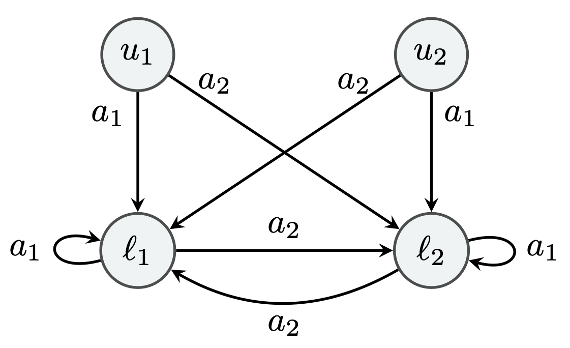
We define the MDP to be as in figure to the right. The state and action spaces are \(\mathcal{S} = \{u_1, l_1, u_2, l_2\}\) and \(\mathcal{A} = \{a_1, a_2\}\). We define \(\mathcal{S}_i = \{u_i, l_i\}\), \(\mathbf{U} = \{u_1, u_2\}\), and \(\mathbf{L} = \{l_1, l_2\}\). In words, for $i\in {1,2}$, action $a_1$ makes the next state to be $l_i$ whenever the initial state is either $l_i$ or $u_i$. On the other hand, action $a_2$ makes the next state $l_i$ when the inital state is either $l_{2-i}$ or $u_{2-i}$. Thus, both actions lead to a state in $\mathbf{L}$, but $a_1$ stays in $\mathcal{S}_i$, while $a_2$ switches from $\mathcal{S}_1$ to $\mathcal{S}_2$ and vice versa.
The reward function is specified in terms of a positive scalar \(r^*>0\) whose value will be chosen later. In particular, we let
\[\begin{align*} r (s, a_1) = \begin{cases} - r^* + 2 \varepsilon, & \text{if $s \in \mathbf{U}$}; \\ - r^*, & \text{if $s \in \mathbf{L}$}; \end{cases} \quad\text{and}\quad r (s, a_2) = 0\,. \end{align*}\]Importantly, the reward is larger at $u_i$ than at $l_i$, which will cause LSPI (with appropriate features) to overestimate the values of states in $\mathbf{L}$. Provided that $r(s,a_1)<0$, equivalently,
\[\begin{align} 2 \varepsilon< r^*\,, \label{eq:c1} \end{align}\]the optimal policy is unique and takes $a_2$ everywhere: Switching incurs no cost, while not switching does.
For any memoryless policy $\pi$, from the Bellman equations for the policy we get that the action-value function of $\pi$ satisfies the following equations:
\[\begin{align*} q^{\pi} (s, a_1) = \begin{cases} - r^* + 2 \varepsilon \mathbb{I} \{s \in \mathbf{U}\} + \gamma v^{\pi} (l_1)\,, & \text{if $s \in \mathcal{S}_1$}\,; \\ - r^* + 2 \varepsilon \mathbb{I} \{s \in \mathbf{U}\} + \gamma v^{\pi} (l_2)\,, & \text{if $s \in \mathcal{S}_2$}\,, \end{cases} \quad q^{\pi} (s, a_2) = \begin{cases} \gamma v^{\pi} (l_2)\,, & \text{if $s \in \mathcal{S}_1$}\,; \\ \gamma v^{\pi} (l_1)\,, & \text{if $s \in \mathcal{S}_2$}\,. \end{cases} \end{align*}\]The feature map we consider is a state-aggregation feature map, where states in $\mathcal{S}_i$ receive the same action-values:
\[\begin{align*} \phi (s, a) = \begin{pmatrix} \mathbb{I} \{s \in \mathcal{S}_1\} \mathbb{I} \{a = a_1\} \\ \mathbb{I} \{s \in \mathcal{S}_1\} \mathbb{I} \{a = a_2\} \\ \mathbb{I} \{s \in \mathcal{S}_2\} \mathbb{I} \{a = a_1\} \\ \mathbb{I} \{s \in \mathcal{S}_2\} \mathbb{I} \{a = a_2\} \end{pmatrix}\,. \end{align*}\]Therefore, the class of greedy policies w.r.t. $\theta^\top \phi$ contains the optimal policy, provided that we keep the rewards of using $a_1$ negative. The action-value function is estimated by
\[\begin{align*} \theta_\pi = \arg\min_{\theta \in \mathbb{R}^d} \sum_{(s, a) \in \mathcal{S} \times \mathcal{A}} \left( \theta^\top \phi (s, a) - q^{\pi} (s, a) \right)^2\,, \end{align*}\]which is the same as minimizing the weighted squared error where the weighting is given by the uniform distribution over $\mathcal{S} \times \mathcal{A}$. Note that the uniform distribution is a $G$-optimal design distribution for this feature map.
By the choice of features, for \(i,j\in \{1,2\}\), $\Phi \theta$ assigns the same value to members of \(\mathcal{S}_i\times \{a_j\}\). Hence, it follows that
\[\begin{align*} \theta_\pi = \frac12 \begin{pmatrix} q^{\pi} (u_1, a_1) + q^{\pi} (l_1, a_1) \\ q^{\pi} (u_1, a_2) + q^{\pi} (l_1, a_2) \\ q^{\pi} (u_2, a_1) + q^{\pi} (l_2, a_1) \\ q^{\pi} (u_2, a_2) + q^{\pi} (l_2, a_2) \end{pmatrix}\,. \end{align*}\]Note that $\theta_\pi$ also minimizes the maximum-error: \(\theta_\pi \in \arg\min_{\theta \in \mathbb{R}^d} \|\theta^\top \Phi - q^{\pi}\|_\infty\). It follows then that
\[\inf_{\theta \in \mathbb{R}^d} \|\theta^\top \Phi - q^{\pi}\|_\infty = \frac12 \max_{1\le i,j\le 2} |q^{\pi}(u_i,a_j)-q^{\pi}(l_i,a_j)| = \varepsilon\,,\]and hence
\[\tilde \varepsilon (M, \phi) = \sup_{\pi \in \Pi_\phi} \inf_{\theta \in \mathbb{R}^d} \|\theta^\top \Phi - q^{\pi}\|_\infty = \varepsilon.\]Consider the policy \(\pi \in \Pi_\phi\) that takes \(a_1\) at states in \(\mathcal{S}_1\) and takes $a_2$ at states in \(\mathcal{S}_2\). By symmetry, the policy $\pi’ \in \Pi_\phi$ that takes $a_2$ at states in \(\mathcal{S}_1\) and takes $a_1$ in states at \(\mathcal{S}_2\) will show a similar behavior. Then,
\[\begin{align*} q^{\pi} (s, a_1) = \begin{cases} - \dfrac{r^*}{1-\gamma} + 2 \varepsilon \mathbb{I} \{s \in \mathbf{U}\}\,, & \text{if $s \in \mathcal{S}_1$}\,; \\ - \dfrac{r^*}{1-\gamma} + 2 \varepsilon \mathbb{I} \{s \in \mathbf{U}\} + \gamma r^*\,, & \text{if $s \in \mathcal{S}_2$}\,, \end{cases} \quad q^{\pi} (s, a_2) = \begin{cases} - \dfrac{\gamma^2 r^*}{1-\gamma}\,, & \text{if $s \in \mathcal{S}_1$}\,; \\ - \dfrac{\gamma r^*}{1-\gamma}\,, & \text{if $s \in \mathcal{S}_2$}\,. \end{cases} \end{align*}\]Therefore,
\[\begin{align*} \theta_\pi^\top = \begin{pmatrix} - \dfrac{r^*}{1-\gamma} + \varepsilon\,, - \dfrac{\gamma^2 r^*}{1-\gamma}\,, - \dfrac{r^*}{1-\gamma} + \varepsilon + \gamma r^*\,, - \dfrac{\gamma r^*}{1-\gamma} \end{pmatrix}\,, \end{align*}\]and thus, for \(\hat{q}_\pi = \Phi \theta_\pi\) we have
\[\begin{align*} \hat{q}_\pi (s, a_1) - \hat{q}_\pi (s, a_2) = \begin{cases} - (1+\gamma) r^* + \varepsilon\,, & \text{if $s \in \mathcal{S}_1$}\,; \\ - (1-\gamma) r^* + \varepsilon\,, & \text{if $s \in \mathcal{S}_2$}\,. \end{cases} \end{align*}\]Hence, if we choose $r^*$ such that
\[\begin{align} -(1+\gamma) r^*+\varepsilon<0 \,, \label{eq:c2} \\ -(1-\gamma) r^*+\varepsilon>0 \,, \label{eq:c3} \end{align}\]then the policy that is greedy with respect to \(\hat{q}_\pi\) will be $\pi’$. Vice versa, the policy that will be greedy with respect to $\hat{q}_{\pi’}$ will be $\pi$. Hence, the idealized version of LSPI switches between $\pi$ and $\pi’$ indefinitely. Conditions \eqref{eq:c2} and \eqref{eq:c3}, together with \eqref{eq:c1}, mean that \(r^*\) should take on a value in the interval $(2\varepsilon,\varepsilon/(1-\gamma))$, which is non-empty since by assumption $\gamma>1/2$. Let us choose the midpoint of this interval for \(r^*\):
\[r^* = \varepsilon+ \frac{\varepsilon}{2(1-\gamma)}\,.\]Now, noting that $v^* = 0$, we have
\[\begin{align*} v^{*} (l_1) - v^{\pi} (l_1) = v^{*} (l_2) - v^{\pi'} (l_2) = \dfrac{r^*}{1-\gamma} \ge \frac{\varepsilon}{2(1-\gamma)^2} \,, \end{align*}\]and the proof is concluded by noting that $v^* \ge v^{\pi},v^{\pi’}$. \(\qquad \blacksquare\)
Thus, the proof reveals that in the MDP constructed in the proof LSPI leads to a sequence of policies that alternate between each other. “Convergence” is fast, yet, the guarantee is far from satisfactory. In particular, in the same example, an alternate algorithm, which we will cover next can reduce the quadratic dependence on the horizon to a linear dependence.
Politex
Politex comes from Policy Iteration with Expert Advice. Assume that one is given a featurized MDP \((M,\phi)\) with state-action feature-map \(\phi\) and access to a simulator, and a $G$-optimal design \(\mathcal{C}\subset \mathcal{S}\times\mathcal{A}\) for \(\phi\).
Politex generates a sequence of policies \(\pi_0,\pi_1,\dots\) such that for \(k\ge 1\),
\[\pi_k(a|s) \propto \exp\left( \eta \bar q_{k-1}(s,a)\right)\,,\]where
\[\bar q_{k} = \hat q_0 + \dots + \hat q_j,\]with
\[\hat q_j = \Pi \Phi \hat \theta_j,\]where for \(j\ge 0\), \(\hat\theta_j\) is the parameter vector obtained by running the least-squares policy evaluation algorithm based on G-optimal design (LSPE-G) to evaluate policy \(\pi_j\) (see this lecture). In particular, recall that this algorithm rolls out policy \(\pi_j\) from the points of a G-optimal design to produce \(m\) independent trajectories of length \(H\) each, calculates the average return for each of these design points and then solves the (weighted) least-squares regression problem where the features are used to regress on the obtained values.
Above, \(\Pi : \mathbb{R}^{\mathcal{S}\times\mathcal{A}} \to \mathbb{R}^{\mathcal{S}\times\mathcal{A}}\) truncates its argument to the \([0,1/(1-\gamma)]\) interval:
\[(\Pi q)(s,a) = \max(\min( q(s,a), 1/(1-\gamma)), 0), \qquad (s,a) \in \mathcal{S}\times \mathcal{A}\,.\]Note that to calculate \(\pi_k(a\vert s)\), one does need to calculate \(E_k(s,a)=\exp\left( \eta \Pi [ \phi(s,a)^\top \bar \theta_{k-1} ] \right)\) and then compute \(\pi_k(a\vert s) = E_k(s,a)/\sum_{a'} E_k(s,a')\).
Unlike in policy iteration, the policy returned by Politex after $k$ iterations is either the “mixture policy”
\[\bar \pi_k = \frac{1}{k} (\pi_0+\dots+\pi_{k-1})\,,\]or the policy which gives the best value with respect to the start state, or start distribution. For simplicity, let us just consider the case when $\bar \pi_k$ is used as the output. The meaning of a mixture policy is simply that one of the $k$ policies is selected uniformly at random and then the selected policy is followed for the rest of time. Homework 3 gives precise definitions and asks you to prove that the value function of $\bar \pi_k$ is just the mean of the value functions of the constituent policies:
\[\begin{align} v^{\bar \pi_k} = \frac{1}{k} \left(v^{\pi_0}+\dots+v^{\pi_{k-1}}\right)\,. \label{eq:avgpol} \end{align}\]We now argue that the dependence on the approximation error of the suboptimality gap of $\bar \pi_k$ only scales with $1/(1-\gamma)$, unlike the case of approximate policy iteration.
For this, recall that by the value difference identity
\[v^{\pi^*} - v^{\pi_j} = (I-\gamma P_{\pi^*})^{-1} \left[T_{\pi^*} v^{\pi_j} - v^{\pi_j} \right]\,.\]Summing up, dividing by $k$, and using \eqref{eq:avgpol} gives
\[v^{\pi^*} - v^{\bar \pi_k} = \frac1k (I-\gamma P_{\pi^*})^{-1} \sum_{j=0}^{k-1} T_{\pi^*} v^{\pi_j} - v^{\pi_j}\,.\]Now, \(T_{\pi^*} v^{\pi_j} = M_{\pi^*} (r+\gamma P v^{\pi_j}) = M_{\pi^*} q^{\pi_j}\). Also, \(v^{\pi_j} = M_{\pi_j} q^{\pi_j}\). Let \(\hat q_j = \Pi \Phi \hat \theta_j\). Elementary algebra then gives
\[\begin{align*} v^{\pi^*} - v^{\bar \pi_k} & = \frac1k (I-\gamma P_{\pi^*})^{-1} \sum_{j=0}^{k-1} M_{\pi^*} q^{\pi_j} - M_{\pi_j} q^{\pi_j}\\ & = \frac1k(I-\gamma P_{\pi^*})^{-1} \underbrace{ \sum_{j=0}^{k-1} M_{\pi^*} \hat q_j - M_{\pi_j} \hat q_j}_{T_1} + \underbrace{\frac1k (I-\gamma P_{\pi^*})^{-1} \sum_{j=0}^{k-1} ( M_{\pi^*} - M_{\pi_j} )( q^{\pi_j}-\hat q_j)}_{T_2} \,. \end{align*}\]We see that the approximation errors $\varepsilon_j = q^{\pi_j}-\hat q_j$ appear only in term $T_2$. In particular, taking pointwise absolute values, using the triangle inequality, we get that
\[\|T_2\|_\infty \le \frac{2}{1-\gamma} \max_{0\le j \le k-1}\| \varepsilon_j\|_\infty\,,\]which shows the promised dependence. It remains to show that \(\|T_1\|_\infty\) above is also under control. However, this is left to the next lecture.
Notes
State aggregation and extrapolation friendliness
The $\sqrt{d}$ in our results comes from controlling the extrapolation errors of linear prediction. In the case of state-aggregretion, however, this extra \(\sqrt{d}\) error amplification is completely avoided: Clearly, if we measure a function with a precision \(\varepsilon\) and there is at least one measurement per part, then by using the value measured at each part (at an arbitrary state there) over the whole part, the worst-case error is bounded by \(\varepsilon\). Weighted least-squares in this context just takes the weighted average of the responses over each part and uses this as the prediction, so it also avoids amplifying approximation errors.
In this case, our analysis of extrapolation errors is clearly conservative. The extrapolation error was controlled in two steps: In our first lemma, for \(\rho\) weighted least-squares we reduced this problem to that of controlling \(g(\rho)=\max_{z\in \mathcal{Z}} \| \phi(z) \|_{G_{\rho}^{-1}}\) where \(G_{\rho}\) is the moment matrix for \(\rho\). In fact, the proof of this lemma is the culprit: By carefully inspecting the proof, we can see that the application of Jensen’s inequality introduces an unnecessary term: For the case of state aggregation (orthonormed feature matrix),
\[\sum_{z' \in C} \varrho(z') |\phi(z')^\top G_\varrho^{-1} \phi(z')| = 1\,\]as long as the design \(\rho\) is such that it chooses any group exactly once. Thus, the case of state-aggregation shows that some feature-maps are more extrapolation friendly than others. Also, note that the Kiefer-Wolfowitz theorem, of course, still gives that \(\sqrt{d}\) is the smallest value that we can get for \(g\) when optimizing for \(\rho\).
It is a fascinating question of how extrapolation errors behave for various feature-maps.
Least-squares value iteration (LSVI)
In homework 2, Question 3 was concerned with least-squares value iteration. The algorithm concerned (call it LSVI-G) uses a random approximation of the Bellman operator, based on a G-optimal design (and action-value functions). The problem was to show a result similar to what holds for LSPI-G holds for LSVI-G, as well. That is, for any MDP feature-map pair $(M,\phi)$ and any $\varepsilon’>0$ excess suboptimality target, with a total runtime of
\[\text{poly}\left( d, \frac{1}{1-\gamma}, A, \frac{1}{\varepsilon'} \right)\,,\]least-squares policy iteration with $G$-optimal design (LSPI-G) can produce a policy $\pi$ such that the suboptimality gap $\delta$ of $\pi$ satisfies
\[\begin{align} \delta \le \frac{4(1+\sqrt{d})}{(1-\gamma)^{\color{red} 2}} \varepsilon_\text{BOO} + \varepsilon'\,. \label{eq:lsviup} \end{align}\]Thus, the dependence on the horizon of the approximation error is similar to the one that was obtained for LSPI. Note that the definition of \(\varepsilon_\text{BOO}\) is different from what we have used in analyzing LSPI:
\[\varepsilon_{\text{BOO}} := \sup_{\theta}\inf_{\theta'} \| \Phi \theta' - T \Pi \Phi \theta \|_\infty\,.\]Above, \(T\) is the Bellman optimality oerator for action-value functions and $\Pi$ is defined so that for \(f:\mathcal{S}\times \mathcal{A}\to \mathbb{R}\), \(\Pi f\) is also a $\mathcal{S}\times \mathcal{A}\to \mathbb{R}$ function which is obtained from $f$ by truncating for each input $(s,a)$ the value $f(s,a)$ to $[0,1/(1-\gamma)]$: $(\Pi(f))(s,a) = \max(\min( f(s,a), 1/(1-\gamma) ), 0)$. In $\varepsilon_{\text{BOO}}$, “BOO” stands for “Bellman-optimality operator” in reference to the appearance of $T$ in the definition.
In general, the error measures \(\varepsilon\) used in LSPI and \(\varepsilon_{\text{BOO}}\) are incomparable. The latter quantity measures a “one-step error”, while \(\varepsilon\) is concerned with approximating functions defined over an infinite-horizon.
Linear MDPs
Call an MDP linear if both the reward function and the next state distributions for each state lie in the span of the features: \(r = \Phi \theta_r\) with some $\theta_r\in \mathbb{R}^d$ and $P$, as an $\mathrm{S}\mathrm{A}\times \mathrm{S}$ matrix takes the form \(P = \Phi W\) with some \(W\in \mathbb{R}^{d\times \mathrm{S}}\). Clearly, this is a notion that captures how well the “dynamics” (including the reward) of the MDP can be “compressed”.
When an MDP is linear, \(\varepsilon_{\text{BOO}}=0\). We also have in this case that $\varepsilon=0$. More generally, defining \(\zeta_r = \inf_{\theta}\| \Phi \theta_r - r \|_\infty\) and \(\zeta_P=\inf_W \|\Phi W - P \|_\infty\), it is not hard to see that \(\varepsilon_{\text{BOO}}\le \zeta_r + \gamma \zeta_P/(1-\gamma)\) and \(\varepsilon\le \zeta_r + \gamma \zeta_P/(1-\gamma)\), which shows that both policy iteration (and its soft versions) and value iteration are “valid” approaches, though, by ignoring the fact that we are comparing upper bounds, this also shows that value iteration may have an edge over policy iteration when the MDP itself is compressible. This should not be too surprising given that value-iteration is “more direct” in aiming to calculate \(q^*\). Yet, they may exist cases when the action-value functions are compressible, while the dynamics is not.
Stationary points of a policy search objective
Let \(J(\pi) = \mu v^\pi\). A stationary point of \(J\) with respect to some set of memoryless policies \(\Pi\) is any \(\pi\in \Pi\) such that
\[\langle \nabla J(\pi), \pi'- \pi \rangle \le 0\,.\]It is known that if $\phi$ are state-aggregation features then any stationary point \(\pi\) of \(J\) satisfies
\[\mu v^\pi \ge \mu v^* - \frac{4\varepsilon_{\text{apx}}}{1-\gamma}\,,\]where $\varepsilon_{\text{apx}}$ is defines as the worst-case error of approximation action-value functions of $\phi$-measurable policies with the features (the same constant as used in the analysis of approximate policy iteration).
Soft-policy iteration with Averaging
Politex can be seen as a “soft” version of policy iteration with averaging. The softness is controlled by $\eta$: When $\eta\to \infty$, Politex uses a greedy policy w.r.t. to an average of all previous \(Q\)-functions. Notice that in this case if Politex were to use a greedy policy w.r.t. the last \(Q\)-function, then it would reduce exactly to LSPI-G. As we have seen, in LSPI-G the approximation error can get quadratically amplified with the horizon $1/(1-\gamma)$. Thus, one way to avoid this quadratic amplification is to stay soft with averaging. As we shall see in the next lecture, the price of this is a relatively slower convergence to a target suboptimality excess value. Nevertheless, the promise is that the algorithm will still stay polynomial in all the relevant quantities.
References
The LSPI lower bound idea came from this paper
- Russo D. Approximation benefits of policy gradient methods with aggregated states. arXiv preprint arXiv:2007.11684. 2020 Jul 22. pdf
Here we have presented a simpler version of the construction which still obtains the same lower bound gaurantees. The simpler construction was inspired by Tadashi Kozuno when he taugh this lecture in Winter 2022.
Politex was introduced in the paper
- POLITEX: Regret Bounds for Policy Iteration using Expert Prediction. Abbasi-Yadkori, Y.; Bartlett, P.; Bhatia, K.; Lazic, N.; Szepesvári, C.; and Weisz, G. In ICML, pages 3692–3702, May 2019. pdf
However, as this paper also notes, the basic idea goes back to the MDP-E algorithm by Even-Dar et al:
- Even-Dar, E., Kakade, S. M., and Mansour, Y. Online Markov decision processes. Mathematics of Operations Research, 34(3):726–736, 2009.
This algorithm considered a tabular MDP with nonstationary rewards – a completely different setting. Nevertheless, this paper introduces the basic argument presented above. The Politex paper notices that the argument can be extended to the case of function approximation. In particular, it also notes the nature of the function approximator is irrelevant as long as the approximation and estimation errors can be tightly controlled.
The Politex paper presented an analysis for online RL and average reward MDPs. Both add significant complications. The argument shown here is therefore a simpler version. Connecting Politex to LSPE-G in the discounted setting is trivial, but has not been presented before in the literature.
The first paper to use the error decomposition shown here together with function approximation is
- Abbasi-Yadkori, Y., Lazic, N., and Szepesvári, C. Modelfree linear quadratic control via reduction to expert prediction. In AISTATS, 2019.