2. The Fundamental Theorem

PDF Version

We start by recapping the definition of MDPs and then firm up the loose ends from the previous lecture: why do the probability distributions \(\mathbb{P}_\mu^\pi\) exist and how are they defined? We then continue with the introduction of what we call the Fundamental Theorem of Dynamic Programming and end with the discussion of value iteration.

Introduction

A Markov decision Process (MDP) is a 5-tuple $M = (\mathcal{S}, \mathcal{A}, P, r, \gamma)$, where $\mathcal{S}$ represents the state space, $\mathcal{A}$ represents the action space, $P = (P_a(s))_{s,a}$ collects the next state distributions for each state-action pair (to represent the transition dynamics), \(r= (r_a(s))_{s,a}\) gives the immediate rewards incurred for taking a given action in a given state, and $0 \leq \gamma < 1$ is the discount factor. As said before, for simplicity, the state set $\mathcal{S}$ and the action set $\mathcal{A}$ are finite.

A policy \(\pi = (\pi_t)_{t \geq 0}\) is an infinite long sequence where for each $t\ge 0$, \(\pi_t: (\mathcal{S} \times \mathcal{A})^{t-1} \times \mathcal{S} \rightarrow \mathcal{M}_1(\mathcal{A})\) assigns a probability distribution to histories of length $t$. (For $\rho\ge 0$ we use $\mathcal{M}_\rho(X)$ to denote the set of nonnegative measures $\mu$ over $X$ that satisfy $\mu(X)=\rho$.) Following a policy in an MDP means that the distribution of the actions in each time step $t\ge 0$ will follow what is prescribed by the policy for whatever the history is at that time.

When a policy is used in an MDP, the interconnection of the policy and the MDP, together with a start-state distribution, results in a distribution $\mathbb{P}$ such that for the infinite long sequence of state-action pairs $S_0,A_0,S_1,A_1,\dots$, $S_0 \sim \mu(\cdot), A_t \sim \pi_t(\cdot | H_t)$, and $S_{t+1} \sim P_{A_t}(S_t)$ for all $t \geq 0$ where $H_t = (S_0,A_0,\dots,S_{t-1},A_{t-1},S_t)$ is the history at time step $t$. This closed loop interaction (or interconnection) of the policy and the MDP is shown in the figure below.

Probabilities over Trajectories

One loose end from the previous lecture was the existence of the probability measures \(\mathbb{P}_\mu^\pi\). For this, we have the following result:

---

Theorem (existence theorem): Fix a finite MDP $M$ with state space $\mathcal{S}$ and action space $\mathcal{A}$. Then there exists a measurable space $(\Omega,\mathcal{F})$ and a sequence of random elements $S_0, A_0, S_1, A_1, \ldots$ over this space, $S_t\in \mathcal{S}$, $A_t\in \mathcal{A}$ for $t\ge 0$, such that for any policy \(\pi = (\pi_t)_{t \geq 0}\) of the MDP $M$ and any probability measure \(\mu \in \mathcal{M}_1(\mathcal{S})\) over $\mathcal{S}$, there exists a probability measure $\mathbb{P}(=\mathbb{P}_{\mu}^{\pi})$ over $(\Omega,\mathcal{F})$ satisfying the following properties:

1. $\mathbb{P}(S_0 = s) = \mu(s)$ for all $s \in \mathcal{S}$,
2. $\mathbb{P}(A_t = a | H_t) = \pi_t(a | H_t)$ for all $a \in \mathcal{A}, t \geq 0$, and
3. $\mathbb{P}(S_{t+1} = s’ | H_t, A_t) = P_{A_t}(S_t, s’)$ for all $s’ \in \mathcal{S}$.

Furthermore, uniqueness holds in the following sense: if \((\tilde{\Omega},\tilde{\mathcal{F}})\) together with \(\tilde S_0,\tilde A_0,\tilde S_1,\tilde A_1,\dots\) also satisfy the conditions of the definition with \({\tilde{\mathbb{P}}}_{\mu}^{\pi}\) denoting the associated probability measures for specific choices of $(\pi,\mu)$ then for any $\pi$, $\mu$, the joint distribution of $S_0,A_0,S_1,A_1,\dots$ under \(\mathbb{P}_\mu^{\pi}\) and that of \(\tilde S_0,\tilde A_0,\tilde S_1,\tilde A_1,\dots\) under \(\tilde{\mathbb{P}}_{\mu}^{\pi}\) are identical.

---

Proof: Use the Ionescu-Tulcea theorem (Theorem 3.3 in the “bandit book”, though the theorem statement there is weaker in that the uniqueness property is left out). \(\qquad\blacksquare\)

Property 3 above is known as the Markov property and is how MDPs derive their name. Note that implicit in the statement of this result is that $\mathcal{S}$ and $\mathcal{A}$ are endowed with the discrete $\sigma$-algebra. This is because we want both ${S_t = s}$ and ${A_t = a}$ to be events for any $s\in \mathcal{S}$ and $a\in \mathcal{A}$ (these appear in the conditions underlying properties 1-3).

Note that the result does not point to any singular measurable space. Indeed, there are many ways to choose $(\Omega,\mathcal{F})$. However, as long as we are only concerned with properties of the distributions of state-action trajectories, thanks to the uniqueness part of the theorem, no ambiguity will arise from this. As a result, in general, we will not care about the choice of $(\Omega,\mathcal{F})$: Any choice as given in the theorem will work. However, for some proofs, it will be convenient to choose $(\mathcal{S}\times \mathcal{A})^{\mathbb{N}}$, the set of infinite long trajectories as $\Omega$, while setting $S_t((s_0,a_0,s_1,a_1,\dots)) = s_t$, $A_t((s_0,a_0,s_1,a_1,\dots)) = a_t$ ($t\ge 0$) and choosing $\mathcal{F}=(2^{\mathcal{S}\times\mathcal{A}})^{\otimes \mathbb{N}}$, which the smallest $\sigma$ algebra that makes $(S_t,A_t)$ measurable for any $t\ge 0$. We will call the resulting probability space the canonical probability space underlying the MDP.

Optimality and Some Notation

As usual, we use $\mathbb{E}$ to denote the expectation operator underlying a probability measure $\mathbb{P}$. When the dependence on $\mu$ or $\pi$ is important, we use $\mathbb{E}_\mu^\pi$. We may drop any of these, when the dropped quantity is clear from the context. We will pay special attention to start state distributions concentrated on a single state. When this is state $s$, the distribution is denoted by $\delta_s$: this is the well-known Dirac distribution with an atom at $s$. The reason we pay special attention to these is because these in a way form the basis of all start state distributions (and in fact quantities that depend linearly on start state distributions). We will use the shorthand \(\mathbb{P}_{s}^{\pi}\) for \(\mathbb{P}_{\delta_s}^{\pi}\). Similarly, we use \(\mathbb{E}_{s}^{\pi}\) for \(\mathbb{E}_{\delta_s}^{\pi}\).

Define the return over a trajectory $\tau = (S_0, A_0, S_1, A_1, \ldots)$ as

\[R = \sum_{t=0}^{\infty} \gamma^t r_{A_t}(S_t).\]

The value function $v^\pi$ of policy $\pi$ maps states to values and in particular for a state $s\in\mathcal{S}$, $v^\pi(s)$ is defined via $v^\pi(s) = \mathbb{E}_{s}^{\pi}[R]$: This is the expected return under the distribution induced by the interconnection of policy $\pi$ and the MDP when the start state is $s$. Note that $v^\pi(s)$ is well-defined. This is because it is the expectation of a quantity that is a function of the trajectory $\tau$; for an explanation see the end-notes.

The standard goal in an MDP is to identify a policy that maximizes this value in every state. A policy achieving this is known as an optimal policy. Whether an optimal policy exists at all is not clear at this stage. In any case, if it exist, an optimal policy must satisfy \(v^\pi = v^*\) where $v^*:\mathcal{S} \to \mathbb{R}$ is defined by

\[v^{*}(s) = \sup_{\pi} v^{\pi}(s)\,, \qquad s\in \mathcal{S}\,.\]

By the definition of the optimal value function, we have \(v^\pi(s) \leq v^{*}(s)\) for all $s \in \mathcal{S}$ and any policy $\pi$. We also use $v^\pi \le v^*$ to express this. In general, $f \le g$ for two functions $f,g$ that are defined over the same domain and take values (say) in the reals, if $f(z)\le g(z)$ holds for all the possible elements $z$ of their common domain. We similarly define $f\ge g$.

We will also identify functions with vectors and allow vector-space operations on them. All vectors, unless otherwise stated, are column vectors. The symbol $\boldsymbol{1}$ is defined as a vector of ones. The length of this vector can change depending on the context. In this lecture, it will be $\mathrm{S}$-dimensional. This symbol will be very useful in a number of calculations. We start with a definition that uses it.

Approximately optimal policies

Let $\varepsilon>0$. A policy $\pi$ is said to be $\varepsilon$-optimal if

\[v^\pi \ge v^* - \varepsilon \boldsymbol{1}\,.\]

Finding an $\varepsilon$-optimal policy with a positive $\varepsilon$ should intuitively be easier than finding an optimal policy.

Memoryless Policies (ML)

If optimal policies would need to remember the past of arbitrary length, it would be hopeless to search for efficient algorithms that can compute them as even describing them could take infinite time. Luckily, this is not the case. In finite MDPs, it will turn out to be sufficient to consider policies that use only the most recent state without losing optimality: this is the subject of the fundamental theorem of MDPs, which we will give shortly. We call the policies that take only the most recent state into account memoryless.

Formally, a memoryless policy can be identified with a map from the states to probability distributions over the actions: \(m: \mathcal{S}\to \mathcal{M}_1(\mathcal{A})\). Given $m$, the memoryless policy, using our previous policy notation, is $\pi_t(a|s_0,a_0,\dots,s_{t-1},a_{t-1},s_t) = m(a|s_t)$, where we abuse notation by using $m(a|s_t)$ in place of $m(s_t)(a)$. Thus, as expected, the policy itself “forgets” the past and just uses the most recent state in assigning probabilities to the individual actions. Under a distribution induced by interconnecting a memoryless policy with an MDP, the sequence of state-action pairs forms a Markov chain.

In what follows, by abusing notation further, when it comes to a memoryless policy, we will identify $\pi$ with $m$ and will just write $\pi: \mathcal{S} \to \mathcal{M}_1(\mathcal{A})$.

For building up to the proof of the fundamental theorem, we start with the concept of discounted occupancy measures.

(Discounted) Occupancy Measure

Given a start state distribution \(\mu \in \mathcal{M}_1(\mathcal{S})\) and a policy \(\pi\), the (discounted) occupancy measure \(\nu_\mu^\pi \in \mathcal{M}_{1/(1-\gamma)}(\mathcal{S} \times \mathcal{A})\) induced by \(\mu\) and \(\pi\) and the underlying MDP \(M\) is defined as

\[\nu_\mu^\pi(s, a) = \sum_{t=0}^\infty \gamma^t \mathbb{P}_\mu^\pi (S_t = s, A_t = a).\]

Interestingly, the value function can be represented as an inner product between the immediate reward function $r$ and the occupancy measure $\nu_\mu^\pi$:

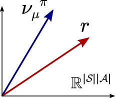
\[\begin{align*} v^\pi(\mu) &= \mathbb{E}_\mu^\pi \left[ \sum_{t=0}^\infty \gamma^t r_{A_t}(S_t) \right] \\ &= \sum_{s, a} \sum_{t=0}^\infty \gamma^t \mathbb{E}_\mu^\pi \left[ r_{A_t}(S_t) \mathbb{I}(S_t = s, A_t = a) \right] \\ &= \sum_{s, a} r_{a}(s) \sum_{t=0}^\infty \gamma^t \mathbb{E}_\mu^\pi \left[ \mathbb{I}(S_t = s, A_t = a) \right] \\ &= \sum_{s, a} r_{a}(s) \sum_{t=0}^\infty \gamma^t \mathbb{P}_\mu^\pi(S_t = s, A_t = a) \\ &= \sum_{s, a} r_a(s) \nu_\mu^\pi(s, a) \\ &=: \langle \nu_\mu^\pi, r \rangle, \end{align*}\]

where $\mathbb{I}(S_t = s, A_t = a)$ is the indicator of the event ${S_t=s,A_t=a}$, which gives the value of one when the event holds (i.e., $S_t = s$ and $A_t = a$), and gives zero otherwise. That the summation over $(s,a)$ can be moved outside of the expectation in the first equality follows because expectations are linear. That the infinite sum can be moved outside is more subtle: this follows from Lebesgue’s dominated convergence theorem. See, for example, Chapter 2 of Lattimore & Szepesvári (2020).

With the above equation, we see that the problem of maximizing the expected reward for a given initial distribution is the same as choosing a policy that “stirs” the occupancy measure to maximally align with the reward vector $r$. A better alignment will result in a higher value for the policy. This is depicted in the figure below.

A key step in proving the sufficiency of memoryless policies for optimal control is the following result:

---

Theorem: For any policy $\pi$ and a start state distribution $\mu \in \mathcal{M}_1(\mathcal{S})$, there exists a memoryless policy $\pi’$ such that

\[\nu_\mu^{\pi'} = \nu_\mu^{\pi}.\]

---

Proof (hint): First define the occupancy measure over the state space \(\tilde{\nu}_\mu^\pi(s) := \sum_a \nu_\mu^\pi(s, a)\). Then show that the theorem statement holds for the policy $\pi’$ defined as follows:

\[\pi'(a | s) = \begin{cases} \frac{\nu_\mu^\pi(s, a)}{\tilde{\nu}_\mu^\pi(s)} & \text{if } \tilde{\nu}_\mu^\pi(s) \neq 0 \\ \pi_0(a) & \text{otherwise,} \end{cases}\]

where \(\pi_0(a) \in \mathcal{M}_1(\mathcal{A})\) is an arbitrary distribution. To do this, expand $\tilde \nu_\mu^\pi$ using the definition of discounted occupancy measures and use algebra.

\[\tag*{$\blacksquare$}\]

Note that it is crucial that the memoryless policy obtained depends on the start state distribution: The reader should try to convince themselves that there are non-memoryless policies whose value function cannot be reproduced by the same memoryless policy at every state.

Bellman Operators, Contractions

The last definitions and results that we need before stating the fundamental theorem concern what are known as Bellman operators.

Fix a memoryless policy $\pi$. Recall that $\mathrm{S}$ is the cardinality (size) of $\mathcal{S}$. First, define $r_\pi(s) = \sum_a \pi(a|s) r_a(s)$ to be the expected reward under policy $\pi$ for a given state $s$. Again, we overload the notation and let $r_\pi \in \mathbb{R}^{\mathrm{S}}$ denote a vector whose $s$th element \((r_\pi)_s = r_\pi(s)\). Similarly, we define $P_\pi(s, s’) := \sum_a \pi(a|s) P_a(s, s’)$ and let $P_\pi \in [0, 1]^{\mathrm{S} \times \mathrm{S}}$ denote the stochastic transition matrix where the element in the \(s\)th row and \(s'\)th column \((P_\pi)_{s, s'} = P_\pi(s, s')\). Note that each row of $P_\pi$ sums to one:

\[P_\pi \mathbf{1} = \mathbf{1}\,.\]

The Bellman/policy evaluation operator underlying $\pi$, $T_\pi: \mathbb{R}^{\mathrm{S}} \rightarrow \mathbb{R}^{\mathrm{S}}$, is defined as

\[\begin{align*} T_\pi v(s) &= \sum_a \pi(a|s) \left \{r_a(s) + \gamma \sum_{s'} P_a(s, s') v(s') \right \} \\ &= \sum_a \pi(a|s) \left \{r_a(s) + \gamma \langle P_a(s), v \rangle \right \} \end{align*}\]

or, in short,

\[T_\pi v = r_\pi + \gamma P_\pi v,\]

where $v \in \mathbb{R}^{\mathrm{S}}$. The Bellman operator performs a one-step lookahead (also called a Bellman lookahead) on the value function. We will use the notations $(T_\pi(v))(s)$, $T_\pi v(s)$, and \((T_\pi v)_s\) interchangeably. $T_\pi$ is also known as the policy evaluation operator for the policy $\pi$.

The Bellman optimality operator $T: \mathbb{R}^{\mathrm{S}} \rightarrow \mathbb{R}^{\mathrm{S}}$ is defined as

\[T v(s) = \max_a \{ r_a(s) + \gamma \langle P_a(s), v \rangle \}.\]

We use \(\|\cdot\|_\infty\) to denote the maximum-norm: \(\| v \|_{\infty} = \max_i |v_i|\). The maximum-norm is a “good friend” of the operators we just defined. This is because stochastic matrices, viewed as operators and “maximizing” are “good friends” of this norm. All this results in the following proposition:

---

Proposition ($\gamma$-contraction of the Bellman Operators): Given any two vectors $u, v \in \mathbb{R}^{\mathrm{S}}$ and any memoryless policy \(\pi\),

1. \(\|T_\pi u - T_\pi v\|_\infty \leq \gamma \|u - v\|_\infty\), and
2. \(\|T u - T v\|_\infty \leq \gamma \|u - v\|_\infty\).

---

The proposition can be proved by elementary algebra and the complete proof can be found in Appendix A.2 of Szepesvári (2010).

For action $a\in \mathcal{A}$, we will find it useful to also define the operator $T_a: \mathbb{R}^{\mathrm{S}} \to \mathbb{R}^{\mathrm{S}}$ which matches $T_\pi$ with the memoryless policy which in every state chooses action $a$. Of course, this operator, being a special case, satisfies the above contraction property as well. This can be seen as performing a one-step lookahead with a fixed action.

From Banach’s fixed point theorem, we get the following corollary:

---

Proposition (Fixed-point iteration): Given any $u \in \mathbb{R}^{\mathrm{S}}$ and any memoryless policy $\pi$,

1. \(v^\pi = \lim_{k\to\infty} T_\pi^k u\) and in particular for any $k\ge 0$, \(\| v^\pi - T_\pi^k u \|_\infty \le \gamma^k \| u - v^\pi \|_\infty\) where \(v^\pi\) is the unique vector/function that satisfies \(T_\pi v^\pi = v^\pi\);
2. \(v_\infty=\lim_{k\to\infty} T^k u\) is well-defined and in particular for any $k\ge 0$, \(\| v_\infty - T^k u \|_\infty \le \gamma^k \| u - v_\infty \|_\infty\). Furthermore, \(v_\infty\) is the unique vector/function that satisfies \(Tv_\infty = v_\infty\).

---

The Fundamental Theorem

Definition: A memoryless policy $\pi$ is greedy w.r.t. to a value function $v: \mathcal{S} \rightarrow \mathbb{R}$ if in every state $s\in \mathcal{S}$, with probability one $\pi$ chooses actions that maximize $(T_a v)(s)=r_a(s) + \gamma \langle P_a(s), v \rangle$.

Note that there can be more than one action that maximizes the (one-step) Bellman lookahead $(T_a v)(s)$ at any given state (in case there are ties). In fact, ties can be extremely common: Just imagine “duplicating an action” in every state (i.e., the new action has the same associated transitions and rewards as the copied one). If the copied one was maximizing the Bellman lookahead at some state, the new action will do the same. Because we have finitely many actions, a maximizing action always exist. Thus, we can always “take” a greedy policy w.r.t. any $v\in \mathbb{R}^{\mathrm{S}}$.

---

Proposition (Characterizing greedyness): A memoryless policy $\pi$ is greedy w.r.t. $v\in \mathbb{R}^{\mathrm{S}}$ if and only if

\[T_\pi v = T v\,.\]

---

With this, we are ready to state what I call the Fundamental Theorem of MDPs:

---

Theorem (Fundamental Theorem of MDPs): The following hold true in any finite MDP:

1. Any policy $\pi$ that is greedy with respect to $v^*$ is optimal: \(v^\pi = v^*\);
2. It holds that \(v^* = T v^*\).

---

The equation $v=Tv$ is known as the Bellman optimality equation and the second part of the result can be stated in words by saying that the optimal value function satisfies the Bellman optimality equation. Also, our previous proposition on fixed-point iteration, where we already came across the Bellman optimality equation, foreshadows a way of approximately computing \(v^*\) that we will get back to after the proof.

Proof: The proof would be easy if we only considered memoryless policies when defining $v^*$. In particular, letting $\text{ML}$ stand for the set of memoryless policies of the given MDP, define

\[\tilde{v}^*(s) = \sup_{\pi \in \text{ML}} v^\pi(s) \quad \text{for all } s \in \mathcal{S}\,.\]

As we shall see soon, it is not hard to show the theorem just with \(v^*\) replaced everywhere with \(\tilde{v}^*\). That is:

1. Any policy $\pi$ that is greedy with respect to $\tilde{v}^*$ satisfies \(v^\pi = \tilde{v}^*\);
2. It holds that \(\tilde{v}^* = T \tilde{v}^*\).

This is what we will show in Part 1 of the proof, while in Part 2 we will show that \(\tilde{v}^*=v^*\). Clearly, the two parts together establish the desired result.

Part 1: The idea of the proof is to first show that \(\begin{align} \tilde{v}^*\le T \tilde{v}^* \label{eq:suph} \end{align}\) and then show that for any greedy policy $\pi$, \(v^\pi \ge \tilde{v}^*\).

The displayed equation follows by noticing that \(v^\pi \le \tilde{v}^*\) holds for all memoryless policies $\pi$ by definition. Applying $T_\pi$ on both sides, using $v^\pi = T_\pi v^\pi$, we get $v^\pi \le T_\pi \tilde{v}^*$. Taking the supremum of both sides over $\pi$ and noticing that $T v = \sup_{\pi \in \text{ML}} T_\pi v$ for any $v$, together with the definition of \(\tilde{v}^*\) gives \(\eqref{eq:suph}\).

Now, take any memoryless policy $\pi$ that is greedy w.r.t. \(\tilde{v}^*\). Thus, \(T_\pi \tilde{v}^* = T \tilde{v}^*\).

Combined with \(\eqref{eq:suph}\), we get

\[\begin{align} \label{eq:start} T_\pi \tilde{v}^* \ge \tilde{v}^*\,. \end{align}\]

Applying $T_\pi$ on both sides and noticing that $T_\pi$ keeps the inequality intact (i.e., for any $u,v$ such that $u\le v$ we get $T_\pi u \le T_\pi v$), we get

\[T_\pi^2 \tilde{v}^* \ge T_\pi \tilde{v}^* \ge \tilde{v}^*\,,\]

where the last inequality follows from \(\eqref{eq:start}\). With the same reasoning we get that for any $k\ge 0$,

\[T_\pi^k \tilde{v}^* \ge T_\pi^{k-1} \tilde{v}^* \ge \dots \ge \tilde{v}^*\,,\]

Now, by our proposition, the fixed-point iteration $T_\pi^k \tilde{v}^*$ converges to $v^\pi$. Hence, taking the limit above, we get

\[v^\pi \ge \tilde{v}^*.\]

This, together with \(v^\pi \le \tilde{v}^*\) shows that \(v^\pi = \tilde{v}^*\).

Finally, $T \tilde{v}^* = T_\pi \tilde{v}^* = T_\pi v^\pi = v^\pi = \tilde{v}^*$.

Part 2: It remains to be shown that \(\tilde{v}^* = v^*\). Let $\Pi$ be the set of all policies. Because $\text{ML}\subset \Pi$, \(\tilde{v}^*\le v^*\). Thus, it remains to show that

\[\begin{align} \label{eq:mlbigger} v^* \le \tilde{v}^*\,. \end{align}\]

To show this, we will use the theorem that guaranteed that for any state-distribution $\mu$ and policy $\pi$ (memoryless or not) we can find a memoryless policy, which we will call for now $\text{ML}(\pi)$, such that $\nu_\mu^\pi = \nu_\mu^{\text{ML}}$. Fix a state $s\in \mathcal{S}$. Applying this result with $\mu = \delta_s$, we get

\[\begin{align*} v^\pi(s) & = \langle \nu_s^\pi, r \rangle \\ & = \langle \nu_s^{\text{ML}(\pi)}, r \rangle \\ & \le \sup_{\pi'\in \text{ML}} \langle \nu_s^{\pi'}, r \rangle \\ & = \sup_{\pi'\in \text{ML}} v^{\pi'}(s) = \tilde{v}^*(s)\,. \end{align*}\]

Taking the supremum of both sides over $\pi$, we get \(v^*(s)= \sup_{\pi\in \Pi} v^\pi(s) \le \tilde{v}^*(s)\). Since $s\in \mathcal{S}$ was arbitrary, we get \(v^*\le \tilde{v}^*\), finishing the proof. \(\qquad\blacksquare\)

A property that came up during the proof that we will repeatedly use is that $T_\pi$ is monotone as an operator. The same holds for $T$. For the record, we state these as a proposition:

---

Proposition (monotonicity of Bellman operators): For any memoryless policy $\pi$, $T_\pi u \le T_\pi v$ holds for any $u,v\in \mathbb{R}^{\mathrm{S}}$ such that $u\le v$. The same also holds for $T$, the Bellman optimality operator.

---

According to the Fundamental Theorem of MDPs, if we have access to the optimal value function \(v^*\), then we can find the optimal policy in an efficient and effective way. We just have to greedify it w.r.t. to the value function: (abusing the policy notation) \(\pi(s) = \arg\max_{a \in \mathcal{A}} \{r_a(s) + \gamma \langle P_a(s), v^* \rangle \} \quad \forall s \in \mathcal{S}\). Such a greedy policy can be found in $O(\mathrm{S}^2 \mathrm{A})$ time.

Hence, if we can efficiently find the optimal value function, we will get an efficient way of computing an optimal policy. This is to be contrasted with the naive approach to finding an optimal policy, which is to enlist all the policies and compare their value functions to find a policy whose value function dominates the value functions of all the other policies.

However, even if we restrict ourselves to just the set of deterministic policies, there are $\Theta(\mathrm{A}^{\mathrm{S}})$ such policies and thus this can be a costly procedure.

As it turns out, for finite MDPs, there is a way to calculate optimal policies in time that is polynomial in $\mathrm{S}$, $\mathrm{A}$, and $1/(1-\gamma)$, avoiding the exponential growth of the naive approach with the size of the state space. Algorithms that can do this belong to the family of dynamic programming algorithms. For our purposes, we call any algorithm a dynamic programming algorithm that uses the idea of keeping track of value of states (that is, uses value functions) while doing its calculations.

The Fundamental Theorem is somewhat surprising: how come that we can find policies whose value function dominates that of all other policies? In a way, the Fundamental Theorem tells us that the set of value functions of all policies in some MDP (as a set in $\mathbb{R}^{\mathrm{S}}$) is very special: It has a “vertex” which dominates all the other value functions. This is quite fascinating. Of course, the key was the Markov property as this gave us the tool to show the result that allowed us to switch from arbitrary policies to memoryless ones.

Value Iteration

By the Fundamental Theorem, \(v^*\) is the fixed point of $T$. By our earlier proposition, which built on the Banach’s fixed point theorem, the sequence \(\{T^k v\}_{k\ge 0}\) converges to \(v^*\) at a geometric rate. In the context of MDPs, the process of repeatedly applying $T$ to some function is called value iteration. The initial function is usually taken to be the all-zero function, which we denote by $\mathbf{0}$, but, of course, if there is a better initial guess on \(v^*\), that guess can also be used at initialization. The next result gives a bound on the number of iterations required to reach an $\varepsilon$-neighborhood (in the max-norm sense) of $v^*$:

---

Theorem (Value Iteration): Consider an MDP with immediate rewards in the $[0,1]$ interval. Pick an arbitrary positive number $\varepsilon>0$. Let $v_0 = \boldsymbol{0}$ and set

\[v_{k+1} = T v_k \quad \text{for } k = 0, 1, 2, \ldots\]

Then, for $k\ge \ln(1/(\varepsilon(1-\gamma))/\ln(1/\gamma)$, \(\|v_k -v^*\|_\infty \le \varepsilon\).

---

Before the proof recall that

\[H_{\gamma,\varepsilon}:= \frac{\ln(1/(\varepsilon(1-\gamma)))}{1-\gamma} \ge \frac{\ln(1/(\varepsilon(1-\gamma)))}{\ln(1/\gamma)}\,.\]

Thus, the effective horizon, $H_{\gamma,\varepsilon}$, whom we met in the first lecture, appeared again. Of course, this is no coincidence.

Proof: By our assumptions on the rewards, $\mathbf{0} \le v^\pi \le \frac{1}{1-\gamma} \mathbf{1}$ holds for any policy $\pi$. Hence, \(\|v^*\|_\infty \le \frac{1}{1-\gamma}\) also holds. By our fixed-point iteration proposition, we get

\[\begin{align*} \|v_k - v^*\|_\infty &\leq \gamma^k \|v^* - \mathbf{0}\|_\infty = \gamma^k \|v^*\|_\infty \leq \frac{\gamma^k}{1 - \gamma} \,. \end{align*}\]

Solving for the smallest $k$ such that \(\gamma^k/(1-\gamma)\le \varepsilon\) gives the result.

\[\tag*{$\blacksquare$}\]

For fixed $\gamma<1$, note the mild dependence of the iteration complexity on the target accuracy $\varepsilon$: we can expect with only a handful iterations to get in a small vicinity of $v^*$. Note also that the total computation cost is $O(\mathrm{S}^2 \mathrm{A}k)$ and the space required is at most $O(\mathrm{S})$, all assuming each value takes up $O(1)$ memory and arithmetic and logic operations also require $O(1)$ time.

Note that accuracy requirement was set up in the form of additive errors. If the value function \(v^*\) is of order $1/(1-\gamma)$ (the maximum possible order), a relative accuracy of order $2$ means setting $\epsilon=0.5/(1-\gamma)$, making the iteration complexity to be $\ln(2)/(1-\gamma)$. However, for controlling the relative error, the more interesting case is when \(v^*\) takes on small values. Here, we see that the complexity may grow unbounded. Later, we will see that in a way this lack of fine-grained error control of value iteration will mean that value iteration is not ideal for calculating exactly optimal policies.

Notes

Value functions are well-defined

As noted in the text, value functions are well-defined despite that the probability space $(\Omega,\mathcal{F},\mathbb{P})$ is not uniquely defined. In fact, for any $f: (\mathcal{S}\times \mathcal{A})^{\mathbb{N}} \to \mathbb{R}$ (measurable) function and for any $(\Omega,\mathcal{F},\mathbb{P})$ and $(\Omega’,\mathcal{F}’,\mathbb{P}’)$ probability spaces, as long as both $\mathbb{P}$ and $\mathbb{P}’$ satisfy the requirements postulated in the existence theorem, \(\int f(\tau(\omega)) \mathbb{P}(d\omega)=\int f(\tau(\omega)) \mathbb{P}'(d\omega)\), or, introducing $\mathbb{E}$ ($\mathbb{E}’$) to denote the expectation operator underlying $\mathbb{P}$ (respectively, $\mathbb{P}’$), \(\mathbb{E}[f(\tau)]=\mathbb{E}'[f(\tau)]\). It also follows that if we only need probabilities and expectations over trajectories, it suffices to choose $(\Omega,\mathcal{F},\mathbb{P})$ as the canonical probability space induced by the state-action space of the MDP at hand.

Other types of MDPs

The obvious question is what survives of all this in other types of MDPs, such as finite-horizon homogenous or inhomogeneous, with or without discounting, total cost (i.e. negative rewards only), or of course the average cost setting? The story is that the arguments can be usually made to work, but this is not entirely automatic. The subject is well-studied and we will give some references and hints later, perhaps even answer some of these questions.

Infinite spaces anyone?

The first thing that changes when we switch to infinite spaces is that we cannot take the assumption that the immediate rewards are bounded for granted. This can cause quite a bit of trouble: $v^\pi$ for some policies can be unbounded, and the same holds for $v^*$. Negative infinite values could be especially “hurtful”. (LQR control is the simplest example where this comes up.)

Another issue is that we cannot take the existence of greedy policies for granted. This happens already when the number of actions is infinite (what is the action that maximizes the reward $r_a(s)=1-1/a$ where $a>0$?). Oftentimes compactness of the action space and continuity assumptions help with this, though, as much of what we will do will be approximate, approximate greedification should be sufficient for most of the time. From this perspective, that greedy actions may not exist is just annoyance.

Finally, when either the state or action space is uncountably infinite, one has to be careful even with the definition of policies. Using a technical term from probability theory, a choice that makes thing work is to restrict policies to be probability kernels. Using this definition means that we need to put measurability structures over both the state and action spaces (this is only crucial when either respective set has a larger than countable cardinality). The main change here is that with policies defined this way, for any $U$ measurable subset of $\mathcal{A}$, $h_t \mapsto \pi_t(U|h_t)$ must be measurable. This allows us then the use of the Ionescu-Tulcea theorem and at least the definitions can be made to work. The next difficulty in this case is that “greedification” may lead to outside of the set of these “measurable policies”, which could prevent the existence of optimal policies (again, if we are contend with approximate optimality, this difficulty disappears). There is a large literature concerned with these issues.

From infinite trajectories to their finite prefixes

Since trajectories are allowed to be infinitely long, we have a nonconstructive result only for the existence of the probability measures induced by the interconnection of policies and MDPs. Oftentimes we need to check whether two probability measures over these infinitely long trajectories coincide. How can this be done? A general result from measure theory says that two measures agree, if they agree on a generator of the underlying $\sigma$-algebra. A convenient generator system for the $\sigma$-algebra over the trajectories (for the canonical probability space) is the cylinder sets that take the form

\[\{s_0\} \times \{a_0\} \times \dots\times \{ s_t \} \times \mathcal{A} \times (\mathcal{S}\times \mathcal{A})^{\mathbb{N}}\]

and

\[\{s_0\} \times \{a_0\} \times \dots\times \{ s_t \} \times \{a_t\} \times (\mathcal{S}\times \mathcal{A})^{\mathbb{N}}\]

for some $s_0,a_0,\dots,s_t,a_t,\dots$. That is, if $\mathbb{P}$ and $\mathbb{P}’$ agree on the probabilities assigned to these sets, they agree everywehere. This makes things a full circle: what this result says is that we only need to check the probabilities assigned to finite prefixes of the infinitely long trajectories. Phew. Since the probabilities assigned to these finite prefixes are a function of $\mu$, $P$ and $\pi$ alone, it follows that there is a unique probability measure over the trajectory space $ (\mathcal{S}\times \mathcal{A})^{\mathbb{N}}$ that satisfies the requirements postulated in the existence theorem. That is, the canonical probability space is uniquely defined.

Optimization with (Discounted) Occupancy Measures

We learned that the value function can be represented as $v^\pi(\mu) = \sum_{s, a} r_a(s) \nu_\mu^\pi(s, a) = \langle \nu_\mu^\pi, r \rangle$. Thus, maximizing the value function for a given initial distribution $\mu$ is equivalent to maximizing the dot product between $\nu_\mu^\pi$ and $r$. Next, we present a concrete example and point out some interesting results.

To keep this example as simple as possible, we introduce some new notation. Let $\mathcal{A}(s)$ represent the set of actions admissable to the state $s \in \mathcal{S}$. We now define the MDP. Let $\mathcal{S} = \{s_1, s_2 \}$, $\mathcal{A}(s_1) = \{a_1, a_2 \}$ and $\mathcal{A}(s_2) = \{a_3 \}$. Also, let

\[\begin{align*} P_{a_1}(s_1, s_1) = 1, &\quad r_{a_1}(s_1) = 1 \\ P_{a_2}(s_1, s_2) = 1, &\quad r_{a_2}(s_1) = 1/2 \\ P_{a_3}(s_2, s_2) = 1, &\quad r_{a_3}(s_2) = 1/2. \end{align*}\]

Our policy $\pi$ can be parametrized by one parameter $p$ as

\[\begin{align*} \pi(a_1|s_1) &= p \\ \pi(a_2|s_1) &= 1 - p \\ \pi(a_3|s_2) &= 1. \end{align*}\]

Finally, we assume $\mu(s_1) = 1$.

We explicitly write out $\nu_\mu^\pi(s, a) = \sum_{t=0}^\infty \gamma^t \mathbb{P}_\mu^\pi (S_t = s, A_t = a)$ for all state-action pairs.

\[\begin{align*} \nu_\mu^\pi(s_1, a_1) &= \sum_{t=0}^\infty \gamma^t p^{t+1} \\ &= p\sum_{t=0}^\infty (\gamma p)^t \\ &= \frac{p}{1-\gamma p} \\ \nu_\mu^\pi(s_1, a_2) &= \sum_{t=0}^\infty \gamma^t p^t (1-p) \\ &= (1-p)\sum_{t=0}^\infty (\gamma p)^t \\ &= \frac{1-p}{1-\gamma p} \\ \nu_\mu^\pi(s_2, a_3) &= \frac{1}{1-\gamma} - \frac{p}{1-\gamma p} - \frac{1-p}{1-\gamma p} \end{align*}\]

Recall, our goal is to maximize $\sum_{s, a} r_a(s) \nu_\mu^\pi(s, a)$. To do this we plug in the above quantities for $r_a(s)$ and $\nu_\mu^\pi(s, a)$

\[\begin{align*} \sum_{s, a} r_a(s) \nu_\mu^\pi(s, a) &= \frac{1-p}{1-\gamma p} + \frac{1}{2} \left( \frac{p}{1-\gamma p} \right) + \frac{1}{2} \left( \frac{1}{1-\gamma} - \frac{p}{1-\gamma p} - \frac{1-p}{1-\gamma p} \right) \\ &= \frac{1}{2} \left( \frac{p}{1-\gamma p} \right) + \frac{1}{2} \left( \frac{1}{1-\gamma} \right). \end{align*}\]

Noting that the function on the right hand side is monotone increasing for $p \in [0, 1]$, so we get that the above quantity is maximized for $p = 1$.

Thus, the optimal policy is

\[\begin{align*} \pi(a_1|s_1) &= 1 \\ \pi(a_2|s_1) &= 0 \\ \pi(a_3|s_2) &= 1. \end{align*}\]

Which, aligns with our intuition that action $a_1$ should always be selected in state $s_1$ since it produces larger reward. Notice how the set of occupancy measures

\[\left\{ (t, (1-\gamma t-t), 1/(1-\gamma)-t-(1-\gamma t-t)) : t \in [0, 1/(1-\gamma)] \right\}\]

is a convex set. This examples shows that optimizing in the space of occupancy measures could be a linear optimization while optimizing with a policy parametrization could be a non-linear optimization.

Fundamental Theorem

I think I have seen Bertsekas and Shreve call the theorem I call fundamental also by the same name. However, this is not quite a standard name. Nevertheless, the result is important and many other things follow from it. In a way, this is the result that is at the heart of all the theory. I think it deserves this name. I have probably read the proof presented here somewhere, but this was a while ago and the source escapes me. In the RL literature people often start with memoryless policies and work with \(\tilde{v}^*\) rather than with \(v^*\). The question whether \(\tilde{v}^*=v^*\) is well-studied and understood, mostly in the control and operations research literature.

The geometry of the space of value functions

An alternative way of seeing the fundamental theorem is as a result concerning the geometry of the space of value functions. Indeed, fix an MDP $M$ and let \(\mathcal{V} = \{ v^\pi \,:\, \pi \text{ is a policy of } M \}\), while let \(\mathcal{V}^{\mathrm{DET}} = \{ v^\pi \,:\, \pi \text{ is a deterministic memoryless policy of } M \}\). The set $\mathcal{V}$ is the set of all value functions of $M$. Both sets are subsets of $\mathbb{R}^{\mathcal{S}}$. Using terminology from multicriteria optimization, the optimal value function, \(v^*\), is the ideal point of $\mathcal{V}$: \(v^*(s) = \sup \{ v(s)\,:\, v\in \mathcal{V} \}\) for all $s\in \mathcal{S}$. Then, the fundamental theorem states that the ideal point of $\mathcal{V}$ belongs to $\mathcal{V}$: \(v^* \in \mathcal{V}\) and in fact \(v^* \in \mathcal{V}^{\mathrm{DET}}\). However, more is known about $\mathcal{V}$:

---

Theorem (existence theorem): Fix a finite MDP $M$. Then $\mathcal{V} \subset \mathbb{R}^{\mathcal{S}}$ is convex. Furthermore, any extreme point of $\mathcal{V}$ belongs to $\mathcal{V}^{\mathrm{DET}}$.

---

This result is due to Dadashi et al. (2019).

Banach’s fixed point theorem

This theorem can be found in Appendix A.1 of my short RL book (Szepesvári, 2010). However, of course, it can be found in many places (the Wikipedia article is also OK). It is worthwhile to spend some time with this theorem to understand its conditions, going back to concepts like Cauchy-sequences (which should perhaps be called sequences with vanishing oscillations) and completeness of the set of real numbers.

References

The references mentioned before:

• Lattimore, T., & Szepesvári, C. (2020). Bandit algorithms. Cambridge University Press.
• Szepesvári, C. (2010). Algorithms for reinforcement learning. Synthesis lectures on artificial intelligence and machine learning, 4(1), 1-103.

The next work (a book chpater) gives a concise yet relatively thorough introduction. The chapter also gives a proof of the fundamental theorem; through the sufficiency of Markov policies. This is done for the discounted and also for a number of alternate criteria.

• Garcia, Frédérick, and Emmanuel Rachelson. 2013. “Markov Decision Processes.” In Markov Decision Processes in Artificial Intelligence, 1–38. Hoboken, NJ USA: John Wiley & Sons, Inc.

A summary of basic results for countable and Borel state-space, and Borel action spaces, with potentially unbounded (from below) reward functions can be found in the next (excellent) paper, which also gives a concise overview of the history of these results:

• Feinberg, Eugene A. 2011. Total Expected Discounted Reward MDPS: Existence of Optimal Policies. In Wiley Encyclopedia of Operations Research and Management Science. Hoboken, NJ, USA: John Wiley & Sons, Inc.

An argument showing the fundamental theorem for the finite-horizon case derived from a general result of David Blackwell can be found in a blog-post of Maxim Raginsky, who gives further pointers, most notable this. David Blackwell has contributed in numerous ways to the foundations of statistics, decision theory, probability theory, and many many other subjects and the importance of his work cannot be overstated.

• Robert Dadashi, Adrien Ali Taïga, Nicolas Le Roux, Dale Schuurmans, Marc G. Bellemare. 2019. The Value Function Polytope in Reinforcement Learning. ICML. arXiv

---