18. Sample complexity in finite MDPs

Let $Z=\mathcal{S}\times \mathcal{A}$ be the set of state-action pairs. A $Z$-design assigns a count to every member of $Z$, that is, to every state-action pair. In the last lecture we saw that

$$n=\tilde{O}\left(\frac{H^6\mathrm{SA}}{{\delta }_{\text{trg}}}\right)$$

samples are sufficient to obtain a ${\delta }_{\text{trg}}$-suboptimal policy with high probability provided that data is generated from a $Z$-design that assigns the same count to each state-action pair and to get a policy one uses the straightforward plug-in approach that estimates the rewards and transitions using empirical estimates and uses the policy that is optimal with respect to the estimated model. Above, the dependence on the number of state-action pairs is optimal, but the dependence on the horizon $H=\frac{1}{1-\gamma }$ is suboptimal. In the first half of this lecture, I sketch how the analysis presented in the previous lecture can be improved to get the optimal cubic dependence, together with a sketch that shows that the cubic dependence is indeed optimal.

In the second half of the lecture, we consider policy-based data collection, or experimental designs, where the goal is to find a near optimal policy from an initial state, where the data consists of trajectories obtained by rolling out the data-collection policy from the said initial state. Here, we will show a lower bound that shows that the sample complexity in this case is at least as large $\mathrm{\Omega }({\mathrm{A}}^{min(\mathrm{S},H)})$, which shows that there exist an exponential separation between both $Z$-designs and policy-based designs, and also between passive and active learning. To see the latter, note that in the presence of a simulator, with only a reset to an initial state, one can use approximate policy iteration with rollouts, or Politex with rollouts, to get a policy that is near-optimal when started from the initial state that one can reset to but with polynomially many samples in $\mathrm{S},\mathrm{A}$ and $H$ (cf. Lecture 8 and Lecture 14).

Improved analysis of the plug-in method: First attempt

The improvement in the analysis of the plug-in method comes from two sources:

1. Using a version of the value-difference identity and avoiding the use of the policy error bound
2. Using Bernstein’s inequality in place of Hoeffding’s inequality

In this section, we focus on the first aspect. The second aspect will be considered in the next section.

We continue to use the same notation as in the previous lecture. In particular, $M$ denotes the “true” MDP, $\hat{M}$ denotes the estimated MDP and we put $\hat{\cdot }$ on quantities related to this second MDP. We further let ${\pi }^{\ast }$ be one of the memoryless optimal policies of $M$. For simplicity, we will assume that the reward function in $\hat{M}$ is the same as in $M$: As we have seen, the higher order term in our error bound came from errors in the transition probability; the simplifying assumption allows us to focus on reducing this term while minimizing clutter. The arguments are easy to extend to the case when $\hat{r}\ne r$.

Let $\hat{\pi }$ be a policy whose suboptimality in $M$ we want to bound. The idea is to bound the suboptimality of $\hat{\pi }$ by its suboptimality in $\hat{M}$ and also by how much value functions for fixed policies differ when we switch from $P$ to $\hat{P}$. In particular, we have

$$\begin{array}{rl}{v}^{\ast }-v^{\hat{\pi }}& =v^{\ast }-{\hat{v}}^{\ast }+{\hat{v}}^{\ast }-v^{\hat{\pi }}\\ \text{(1)}& & \le v^{{\pi }^{\ast }}-{\hat{v}}^{{\pi }^{\ast }}+\underset{\text{opt. error}}{\underbrace{{\hat{v}}^{\ast }-{\hat{v}}^{\hat{\pi }}}}+{\hat{v}}^{\hat{\pi }}-v^{\hat{\pi }},\end{array}$$

where ${\hat{\pi }}^{\ast }$ denotes an optimal policy in $\hat{M}$ and the inequality holds because ${\hat{v}}^{\ast }={\hat{v}}^{{\hat{\pi }}^{\ast }}\ge {\hat{v}}^{{\pi }^{\ast }}$. The term marked as “opt. error” is the optimization error that arises when $\hat{\pi }$ is not (quite) optimal in $\hat{M}$. This term is controlled by the choice of $\hat{\pi }$. For simplicity, assume for now that $\hat{\pi }$ is an optimal policy in $\hat{M}$, so that we can drop this term. We further assume that $\hat{\pi }$ is a deterministic optimal policy of $\hat{M}$.

It remains to bound the first and last terms. Both of these terms have the form $v^{\pi }-{\hat{v}}^{\pi }$, i.e., the difference between the value functions of the same policy $\pi$ in the two MDPs (here, $\pi$ is either ${\pi }^{\ast }$ or $\hat{\pi }$). This difference, similar to the value difference identity, can be expressed as a function of the difference $P-\hat{P}$, as shown in the next result:

---

Lemma (value difference from transition differences): Let $M$ and $\hat{M}$ be two MDPs sharing the same state-action space, rewards, but differing in their transition probabilities. Let $\pi$ be a memoryless policy over the shared state-action space of the two MDPs. Then, the following identities holds:

$$\begin{array}{}\text{(2)}& v^{\pi }-{\hat{v}}^{\pi }& =\gamma \underset{\delta ({\hat{v}}^{\pi })}{\underbrace{(I-\gamma P_{\pi }{)}^{-1}{M}_{\pi }(P-\hat{P}){\hat{v}}^{\pi }}},\text{(3)}& {\hat{v}}^{\pi }-v^{\pi }& =\gamma \underset{\hat{\delta }(v^{\pi })}{\underbrace{(I-\gamma {\hat{P}}_{\pi }{)}^{-1}{M}_{\pi }(\hat{P}-P)v^{\pi }}}.\end{array}$$

---

Proof: We only need to prove $\text{(2)}$ since $\text{(3)}$ follows from this identity by symmetry. Concerning the proof of $\text{(2)}$, we start with the closed form expression for value functions. From this we get

$$\begin{array}{r}{v}^{\pi }-{\hat{v}}^{\pi }=(I-\gamma P_{\pi }{)}^{-1}{r}_{\pi }-(I-\gamma {\hat{P}}_{\pi }{)}^{-1}{r}_{\pi }.\end{array}$$

Inspired by the elementary identity that states that $\frac{1}{1-x}-\frac{1}{1-y}=\frac{x-y}{(1-x)(1-y)}$, we calculate

$$\begin{array}{rl}{v}^{\pi }-{\hat{v}}^{\pi }& =(I-\gamma P_{\pi }{)}^{-1}[(I-\gamma {\hat{P}}_{\pi })-(I-\gamma P_{\pi })](I-\gamma {\hat{P}}_{\pi }{)}^{-1}{r}_{\pi }\\ & =\gamma (I-\gamma P_{\pi }{)}^{-1}[P_{\pi }-{\hat{P}}_{\pi }](I-\gamma {\hat{P}}_{\pi }{)}^{-1}{r}_{\pi }\\ & =\gamma (I-\gamma P_{\pi }{)}^{-1}{M}_{\pi }[P-\hat{P}]{\hat{v}}^{\pi },\end{array}$$

finishing the proof. $◼$

Note that in $\text{(3)}$, the empirical transition kernel $\hat{P}$ appears through its inverse by left-multiplying $M_{\pi }(\hat{P}-P)$, while in $\text{(2)}$, through ${\hat{v}}^{\pi }$, it appears by right-multiplying the same deviation term. In the remainder of this section we use $\text{(3)}$, but in the next section we will use $\text{(2)}$.

Combining $\text{(3)}$ with our previous inequality, we immediately get that

$$\begin{array}{}\text{(4)}& v^{\ast }-v^{\hat{\pi }}& \le \frac{\gamma }{1-\gamma }[\Vert (P-\hat{P})v^{{\pi }^{\ast }}{\Vert }_{\mathrm{\infty }}+\Vert (P-\hat{P})v^{\hat{\pi }}{\Vert }_{\mathrm{\infty }}].\end{array}$$

Assume that $\hat{P}$ is obtained by sampling $m$ next states at each state-action pair. By Hoeffding’s inequality and a union bound over the state-action pairs, for any fixed $v\in [0,H{]}^{SA}$ and $0\le \zeta <1$, with probability $1-\zeta$, we have

$$\begin{array}{}\text{(5)}& \Vert (P-\hat{P})v{\Vert }_{\mathrm{\infty }}=H\sqrt{\frac{\log (SA/\zeta )}{2m}}\end{array}$$

and in particular with $v=v^{{\pi }^{\ast }}$, we have

$$\Vert (P-\hat{P})v^{{\pi }^{\ast }}{\Vert }_{\mathrm{\infty }}=\tilde{O}\left(H/\sqrt{m}\right).$$

Controlling the second term in $\text{(4)}$ requires more care as $\hat{\pi }$ is random and depends on the same data that is used to generate $\hat{P}$. To deal with this term, we use another union bound. Let $\tilde{V}=\{v^{\pi }:\pi :\mathcal{S}\to \mathcal{A}\}$ be the set of all possible value functions that we can obtain by considering deterministic policies. Since by construction $\hat{\pi }$ is also a deterministic policy, ${\hat{v}}^{\hat{\pi }}\in \tilde{V}$. Hence,

$$\Vert (P-\hat{P}){\hat{v}}^{\hat{\pi }}{\Vert }_{\mathrm{\infty }}\le \underset{v\in \tilde{V}}{sup}\Vert (P-\hat{P})v{\Vert }_{\mathrm{\infty }}.$$

and thus by a union bound over the $|\tilde{V}|\le A^S$ functions $v$ in $\tilde{V}$, we get that with probability $1-\zeta$,

$$\begin{array}{rl}\Vert (P-\hat{P}){\hat{v}}^{\hat{\pi }}{\Vert }_{\mathrm{\infty }}& \le H\sqrt{\frac{\log (SA|\tilde{V}|/\zeta )}{2m}}=H\sqrt{\frac{\log (SA/\zeta )+S\log (A)}{2m}}=\tilde{O}\left(H\sqrt{S/m}\right).\end{array}$$

Putting things together, we see that

$$v^{\ast }-v^{\hat{\pi }}=\tilde{O}\left(H^2\sqrt{S/m}\right),$$

which reduces the dependence on $H$ of the sample size bound from $H^6$ to $H^4$. As we shall see soon, this is not the best possible dependence on $H$. This method also falls short of giving the best possible dependence on the number of states. In particular, inverting the above bound, we see that with this method we can only guarantee a $\delta$-optimal policy if the total number of samples, $n=SAm$ is at least

$$\tilde{O}(S^{2}A{H}^4/{\delta }^2)$$

while below we will see that the optimal bound is $\tilde{O}(SA{H}^3/{\delta }^2)$.

Improved analysis of the plug-in method: Second attempt

There are two further ideas that help one achieve the sample complexity which will be seen to be optimal. One is to use what is known as Bernstein’s inequality in place of Hoeffding’s inequality, together with a clever observation on the “total variance” and the second is to improve the covering argument. The first idea helps with improving the horizon dependence, the second helps with improving the dependence on the number of states. In this lecture, we will only cover the first idea and sketch the second.

Bernstein’s inequality is a classic result in probability theory:

---

Theorem (Bernstein’s inequality): Let $b>0$ and let $X_1,\dots ,X_m\in [0,b]$ be an i.i.d. sequence and define ${\overline{X}}_m$ as the sample mean of this sequence: ${\overline{X}}_m=\frac{1}{m}(X_1+\cdots +X_m)$. Then, for any $\zeta \in (0,1)$, with probability at least $1-\zeta$,

$$|{\overline{X}}_m-\mathbb{E}[X_1]|\le \sigma \sqrt{\frac{2\log (2/\zeta )}{m}}+\frac{2}{3}\frac{b\log (2/\zeta )}{m},$$

where ${\sigma }^2=\text{Var}(X_1)$.

---

To set expectations, it will be useful to compare this bound to Hoeffding’s inequality. In particular, in the setting of the lemma Hoeffding’s inequality also applies and gives

$$|{\overline{X}}_m-\mathbb{E}[X_1]|\le b\sqrt{\frac{\log (2/\zeta )}{2m}}.$$

Since in our case $b=H$ (the value functions take values in the $[0,H]$ interval), using $m=H^3/{\delta }^2$ (which would give rise to the optimal sample size), Hoeffding’s inequality gives a bound of size $H{H}^{-3/2}\delta =H^{-1/2}\delta$ (cf. $\text{(5)}$). This is a problem: Ideally, we would like to see $H^{-1}\delta$ here, because inequality \cref{eq:vdeb} introduces an additional $H$ factor.

We immediately see that for Bernstein’s inequality to make a difference, just focusing on the first term in Bernstein’s inequality, we need $\sigma =O(H^{1/2})$. In fact, since $b/m=H^{-2}{\delta }^2=o(H^{-1}\delta )$, we see that this is also sufficient to take off the $H$ factor from the sample complexity bound. It thus remains to be seen whether the variance could indeed be this small.

To find this out, fix a state-action pair $(s,a)$ and let $S_1^{\prime },\dots ,S_m^{\prime }\sim P_a(s)$ be an i.i.d. sequence of next states at $(s,a)$. Then, $((\hat{P}-P)v^{\pi })(s,a)=({\hat{P}}_a(s)-P_a(s))v^{\pi }$ has the same distribution as

$$\mathrm{\Delta }(s,a)=\frac{1}{m}\sum _{i=1}^m{v}^{\pi }(S_i^{\prime })-P_a(s)v^{\pi }.$$

Defining $X_i=v^{\pi }(S_i^{\prime })$ and ${\sigma }_{\pi }^2(s,a)=\mathrm{Var}(X_1)$, we see that it is ${\sigma }_{\pi }(s,a)$ that appears when Bernstein’s inequality is used to bound $((\hat{P}-P)v^{\pi })(s,a)$. It remains to be seen how large values ${\sigma }_{\pi }(s,a)$ can take on. Sadly, one can quickly discover that the range of ${\sigma }_{\pi }(s,a)$ is sometimes also as large as $H$. Is Bernstein’s inequality a dead-end then?

Of course, it is not, otherwise we would not have introduced it. In particular, a better bound is possible by directly bounding the maximum-norm of

$$\delta (v^{\pi })=(I-\gamma P_{\pi }{)}^{-1}{M}_{\pi }(P-\hat{P})v^{\pi },$$

which is close to the actual term that we need to bound. Indeed, by \cref{$\text{(2)}$} from the value difference lemma, $v^{\pi }-{\hat{v}}^{\pi }=\gamma \delta ({\hat{v}}^{\pi })$ and thus

$$v^{\pi }-{\hat{v}}^{\pi }=\gamma \delta (v^{\pi })+\gamma (\delta ({\hat{v}}^{\pi })-\delta (v^{\pi })).$$

The second term on the right-hand side is of order $1/m$ (since $(P-\hat{P})({\hat{v}}^{\pi }-v^{\pi })$ appears there and both $P-\hat{P}$ and ${\hat{v}}^{\pi }-v^{\pi }$ have been seen to be of order $1/\sqrt{m}$). As we expect $\delta (v^{\pi })$ to be of order $1/\sqrt{m}$, we will focus on this term.

For simplicity, take now the case when $\pi$ is a fixed, nonrandom policy (we need to bounded $\delta (v^{\pi })$ for $\pi ={\pi }^{\ast }$ and also for $\pi =\hat{\pi }$, the second of which is random). In this case, by a union bound and Bernstein’s inequality, with probability $1-\zeta$,

$$\begin{array}{rl}|(P-\hat{P})v^{\pi }|& \le \sqrt{\frac{2\log (2SA/\zeta )}{m}}{\sigma }_{\pi }+\frac{2H}{3}\frac{\log (2/\zeta )}{m}\mathbf{1}.\end{array}$$

Multiplying both sides by $(I-\gamma P_{\pi }{)}^{-1}{M}_{\pi }$, using a triangle inequality and the special properties of $(I-\gamma P_{\pi }{)}^{-1}{M}_{\pi }$, we get

$$\begin{array}{rl}|\delta (v^{\pi })|& \le (I-\gamma P_{\pi }{)}^{-1}{M}_{\pi }|(P-\hat{P})v^{\pi }|\\ \text{(6)}& & \le \sqrt{\frac{2\log (2SA/\zeta )}{m}}(I-\gamma P_{\pi }{)}^{-1}{M}_{\pi }{\sigma }_{\pi }+\frac{2H^2}{3}\frac{\log (2SA/\zeta )}{m}\mathbf{1}.\end{array}$$

The following beautiful result, whose proof is omitted, gives an $O(H^{3/2})$ bound on the first term appearing on the right-hand side of the above display:

---

Lemma (total discounted variance bound): For any discounted MDP $M$ and policy $\pi$ in $M$, $\Vert (I-\gamma P_{\pi }{)}^{-1}{M}_{\pi }{\sigma }_{\pi }{\Vert }_{\mathrm{\infty }}\le \sqrt{\frac{2}{(1-\gamma {)}^3}}.$

---

Since the bound that we get from here is $H^{3/2}$ and not $H^2$, “we are saved”. Indeed, plugging this into $\text{(6)}$ gives

$$\Vert \delta (v^{\pi }){\Vert }_{\mathrm{\infty }}\le 2\sqrt{\frac{H^3\log (2SA/\zeta )}{m}}+\frac{2H^2}{3}\frac{\log (2SA/\zeta )}{m},$$

which holds with probability $1-\zeta$. Choosing $m=H^3/{\delta }^2$, we see that both terms are $O(\delta )$. It remains to show that a similar result holds for $\pi =\hat{\pi }$. If we use the union bound that we used before, we introduce an extra $S$ factor. Avoiding this extra $S$ factor requires new ideas, but with these we get the following result:

---

Theorem (upper bound for $Z$-designs): Let $\hat{\pi }$ be an optimal policy in the MDP whose transition kernel is $\hat{P}$, a kernel estimated based on a sample of $m$ next states from each state-action pair. Letting $0\le \zeta <1$ and $0\le \delta \le \sqrt{H}$, if

$$m\ge \frac{c\gamma H^3\log (SAH/\delta )}{{\delta }^2}$$

then with probability $1-\zeta$, $\hat{\pi }$ is $\delta$-optimal, where $c$ is a universal constant. In short, for any $0\le \delta \le \sqrt{H}$ there exist an algorithm that produces a $\delta$-optimal policy from a total number of

$$\tilde{O}\left(\frac{\gamma SA{H}^3}{{\delta }^2}\right)$$

samples under a uniform $Z$-design.

---

It remains to be seen whether the same sample complexity holds for larger values of $\delta$, e.g., for $\delta =H/2$.

Lower bound for $Z$-designs

A natural question is whether we can improve on the $H^{3}SA/{\delta }^2$ upper bound, or whether this can be matched by a lower bound. For this, we have the following result:

---

Theorem (lower bound for $Z$-designs): Any algorithm that uses $Z$-designs and is guaranteed to produce a $\delta$-optimal policy needs at least $\mathrm{\Omega }(H^{3}SA/{\delta }^2)$ samples.

---

Proof (sketch): As we have seen in the proof of the upper bound, the key to achieve the cubic dependence was that the sample mean ${\overline{X}}_m$ of $m$ i.i.d. bounded random variables is within a distance of $\sigma \sqrt{1/m}$ to the true mean. In a way, the converse of this is also true: It is “quite likely” that the distance between the sample and true mean is this large. This is not too hard to see for specific distributions, such as when the $X_i$ are normally distributed, or when $X_i$ are Bernoulli distributed (in a way, this is the essence of the central-limit theorem, though the central-limit theorem is restricted for $m\to \mathrm{\infty }$).

So how can we use this to establish the lower bound? In an MDP the randomness comes either from the rewards or the transitions. But in the upper bound above, the rewards were given, so the only source of randomness is transitions. Also, the cubic dependence must hold even if the number of states is a constant. What all this implies is that somehow learning the transition structure with a few states is what makes the sample complexity large as $\gamma \to 1$ (or $H\to \mathr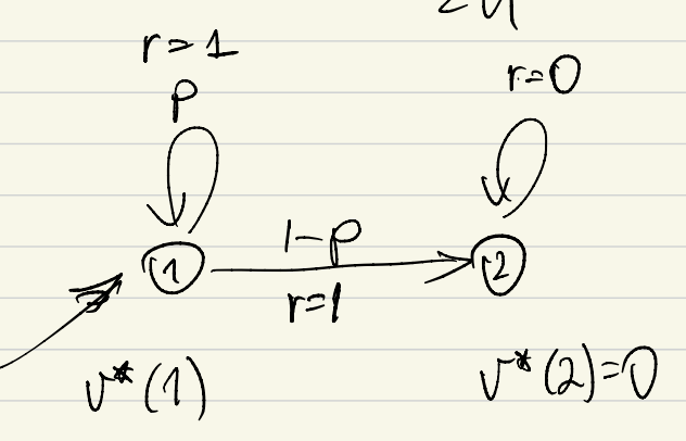m{\infty }$). Clearly, this can only happen if the (small) MDP has self-loops. The smallest example of an MDP with a self-loop is if one has an action and state such that taking that action from that state leads to same action with some positive probability, while with the complementary probability the next state is some other state. This leads to the structure shown on the figure on the right.

As can be seen, there are two states. The transition at the first state, call it state $1$, is stochastic and leads to itself with probability $p$, while it leads to state $2$ with probability $1-p$. The reward associated with both transitions is $1$. The second state, call it state $2$, has a self-loop. The reward associated with this transition is zero.

There are no actions (alternatively, there is only one action at both states). However, if we can show that in the lack of knowledge of $p$, estimating the value of state $1$ up to a precision of $\delta$ takes $\mathrm{\Omega }(H^3/{\delta }^2)$ samples, the sample complexity result will follow. In particular, if we repeat the transition structure $A$ times (sharing the same two states), one can make the value of $p$ for one of this actions ever slightly so different from the others so that its value differs by (say) $2\delta$ from the others. Then, by construction, a learner who uses fewer than $\mathrm{\Omega }(A{H}^3/{\delta }^2)$ total samples at state $1$ will not be able to reliably tell the difference between the value of the special action and the other actions, hence, will not be to choose the right action and will thus be unable to produce a $\delta$-optimal policy. To also add the state dependence, the structure can then be repeated $S$ times.

So it remains to be seen whether the said sample complexity result holds for estimating the value of state $1$. Rather than giving a formal proof, we give a quick heuristic argument, hoping that readers will find this more intuitive.

The starting point for this heuristic argument is the general observation that sample complexity questions concerning estimation problems are essentially questions about the sensitivity of the quantity to be estimated to the unknown parameters. Here, sensitivity means how much the quantity changes if we change the underlying parameter. This sensitivity for small deviations and a single parameter is exactly the derivative of the quantity of interest with respect to the parameter.

In our special case, the value of state $1$, call it $v_p(1)$ (also showing the dependence on $p$) is the quantity to be estimated. Since the value of state $2$ is zero, $v_p(1)$ must satisfy $v_p(1)=p(1+\gamma v_p(1))+(1-p)1$. Solving this we get

$$v_p(1)=\frac{1}{1-p\gamma }.$$

The derivative of this with respect to $p$ is

$$\frac{d}{dp}{v}_p(1)=\frac{\gamma }{(1-\gamma p{)}^2}.$$

To get a $\delta$-accurate estimate of $v_{p_0}(1)$, we need

$$\begin{array}{rl}\delta & \ge |v_{p_0}(1)-v_{{\overline{X}}_m}(1)|\approx \frac{d}{dp}{v}_p(1){|}_{p=p_0}|p_0-{\overline{X}}_m|=\frac{\gamma }{(1-\gamma p_0{)}^2}|p_0-{\overline{X}}_m|\\ & \approx \frac{\gamma }{(1-\gamma p_0{)}^2}\sqrt{\frac{p_0(1-p_0)}{m}}.\end{array}$$

Inverting for $m$, we get that

$$m\gtrsim \frac{{\gamma }^2{p}_0(1-p_0)}{(1-\gamma p_0{)}^4{\delta }^2}.$$

It remains to choose $p_0$ as a function of $\gamma$ to show that the above can be lower bounded by $1/(1-\gamma {)}^3$. If we choose $p_0=\gamma$, we have $1-\gamma p_0=1-{\gamma }^2=(1-\gamma )(1+\gamma )\le 2(1-\gamma )$ and hence

$$\frac{{\gamma }^2{p}_0(1-p_0)}{(1-\gamma p_0{)}^4{\delta }^2}\ge \frac{{\gamma }^2\gamma (1-\gamma )}{2^4(1-\gamma {)}^4{\delta }^2}=\frac{{\gamma }^3}{2^4(1-\gamma {)}^3{\delta }^2}.$$

Putting things together finishes the proof sketch. $◼$

A homework problem is included which explains how to fill in the gaps in the last section of the proof, while pointers to the literature are given that one can use to figure out how to fill the remaining gaps.

Policy-based designs

When the data is generated by following some policy, we talk about policy based designs. Here, the design decision is what policy to use to generate the data. The sample complexity of learning with policy based designs is the number of observations necessary and sufficient for some algorithm to figure out a policy of a fixed target suboptimality, from a fixed initial state, based on data generated by following a policy where the MDP where the policy is followed can be any of the MDPs within the class.

Three questions arise then. (i) The first question (the design question) is what policy to follow during data collection. If the policy can use the full history, the problem is not much different than online learning, which we will consider later. From this perspective the interesting (and perhaps more realistic) case is when the data-collection policy is memoryless and is fixed before the data collection begins. Hence, in what follows, we will restrict our attention to this case. (ii) The second question is what algorithm to use to compute the policy given the data generated. (iii) The final, third question is how large is the sample complexity of learning with policy induced data for some fixed MDP class.

Learning and estimating a good policy from policy induced data is much closer to reality than the same problem from $Z$-designs. Practical problems, such as problems in health care, robotics, etc., are so that we can obtain data generated by following some fixed policy, while it is usually not possible to demand obtaining sample transitions from arbitrary state-action pairs.

For simplicity, let us still consider the case of finite state-action MDPs, but to further simplify matters, let us now consider (homogenous kernel) finite horizon problems with a horizon $H$. As it turns out, the plug-in algorithm of the previous section is still a good algorithm in the sense that it achieves the optimal (minimax) sample complexity. However, the minimax sample complexity is much higher than it is for $Z$-designs:

---

Theorem (sample complexity lower bound with policy induced data): For any $S,A,H$, $0\le \delta$, any (memoryless) data collection policy $\pi$ over the state-action spaces $[S]$ and $[A]$, for any $n\le c{A}^{min(S-1,H)}/{\delta }^2$ and any algorithm $\mathcal{L}$ that maps data that has $n$ transitions to a policy there exist an MDP $M$ with state space $[S]$ and action space $[A]$ such that with constant probability, the policy $\hat{\pi }$ produced by $\mathcal{L}$ is not $\delta$-optimal with respect to the $H$-horizon total reward criterion when the algorithm is fed with data by following $\pi$ in $M$.

---

Proof (sketch): Without loss of generality assume that $S=H+1$; if there are more states, just ignore them, while if there are fewer states then just decrease $H$. Consider an MDP where states $1,\dots ,H$ are organized in a chain under the effect of some actions, and state $H+1$ is an absorbing state with zero associated reward. 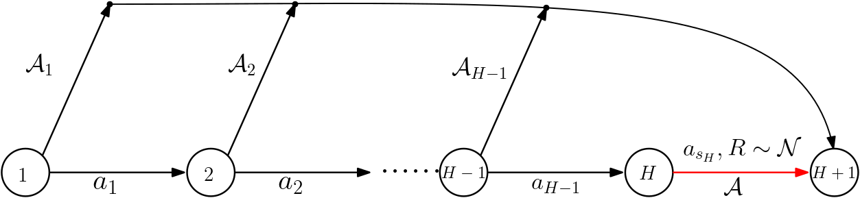For $1\le i\le H$, let action $a_i$ be the one that gets to be chosen with the smallest probability in state $i$ under the data generating policy $\pi$: $a_i=\arg \underset{a\in [A]}{min}\pi (a|i)$. We choose action $a_i$ as the action that moves the state from $i$ to $i+1$, deterministically. Any other action leads to state $H+1$, deterministically. All rewards are zero, except when transitioning from state $H$ to state $H+1$ under action $a_H$, where the reward is stochastic with a normal distribution with mean $\mu$ either $-2\delta$ or $+2\delta$ and a variance of one. The structure of the MDP is shown on the figure in the left-hand side.

Now, because of the choice of $a_i$, $\pi (a_i|i)\le 1/A$. Hence, the probability that starting from state $1$, following policy $\pi$ for $H$ steps will generate the sequence of states $1,2,\dots ,H,H+1$, including the critical transition from state $H$ to state $H+1$, is at most $(1/A{)}^H$. This transition is critical in the sense is that only data from this transition decides whether in state $1$ it is worth taking action $a_1$ or not. In particular, if $\mu =-2\delta$, taking $a_1$ is a poor choice, while if $\mu =2\delta$, taking $a_1$ is the optimal choice. The expected number of times this critical transition is seen is at most $m=n(1/A{)}^H$. With $m$ observations, the value of $\mu$ will be estimated up to an accuracy of $O(\sqrt{1/m})$. When this is smaller than $2\delta$, with constant probability, the sign of $\mu$ cannot be decided and thus with constant probability, any algorithm will fail to identify whether $a_1$ should be taken in state $1$ or not (with a probability, of say, at least $1/2$). Plugging in the expected value of $m$, we get that the condition on $n$ is that $\sqrt{c{A}^H/n}\le 2\delta$ where $c>0$ is some universal constant. Equivalently, the condition is that $n\ge c{A}^H/(4{\delta }^2)$, which is the statement to be proven. $◼$

The lower bound construction suggests that the best policy to be used in the lack of extra information about the MDPs is the uniform policy. Note that a similar statement holds for the discounted setting. The contrast between this lower bound and the polynomial upper bound of the previous section are in strike contrast: Data obtained from following policies can be very poor. One may wonder whether the situation can be improved assuming that the data is obtained from a good policy (say, $2\delta$ optimal policy), but the proof of the previous result in fact shows that this is not the case.

While the exponential lower bound on the sample complexity of learning from policy induced data is already bad enough, one may worry that the situation could be even worse. Could it happen that even the best algorithm needs double exponential number of samples? Or even infinite? A moment of thought shows that the latter is the case is switch to the average reward setting: This is because in the average reward setting the value of an action can depend on the value of a state whose hitting probability within an arbitrary fixed number of transitions is positive, just arbitrarily low. Can something similar happen perhaps in the finite-horizon setting, or the discounted setting? As it turns out, the answer is no. The previous lower bound gives the correct order of the sample complexity of finding a near-optimal policy using policy induced data:

---

Theorem (sample complexity upper bound with policy induced data): With $m=\mathrm{\Omega }(S^3{H}^4{A}^{min(H,S-1)+2}/{\delta }^2)$ episodes of length $H$ collected with the uniform policy from a fixed initial distribution $\mu$, with a constant probability, the plug-in algorithm produces a policy that is $\delta$-optimal when started from $\mu$.

---

Proof (sketch): For simplicity assume that the reward function is known. Let ${\pi }_{\log }$ be the logging policy, which is uniform. Again, assume that the plug-in algorithm produces a deterministic policy.

The proof is based on the decomposition of the suboptimality gap of the policy $\hat{\pi }$ produced that was used before. In particular, by $\text{(1)}$,

$$\begin{array}{}\text{(7)}& v^{\ast }(\mu )-v^{\hat{\pi }}(\mu )& \le v^{{\pi }^{\ast }}(\mu )-{\hat{v}}^{{\pi }^{\ast }}(\mu )+{\hat{v}}^{\hat{\pi }}(\mu )-v^{\hat{\pi }}(\mu ),\end{array}$$

where as before, ${\hat{v}}^{\pi }$ denotes the value function of policy $\pi$ in the empirically estimated MDP. Further, we also used $v(\mu )$ as a shorthand for $\sum _s\mu (s)v(s)(=⟨\mu ,v⟩)$, where $v:[S]\to \mathbb{R}$,

One then needs a counterpart of the value difference lemma. In this case, the following version is convenient: For any policy $\pi$,

$$q_H^{\pi }-{\hat{q}}_H^{\pi }=\sum _{h=0}^{H-1}(P_{\pi }{)}^h(P-\hat{P}){\hat{v}}_{H-h-1}^{\pi },$$

and

$${\hat{q}}_H^{\pi }-q_H^{\pi }=\sum _{h=0}^{H-1}({\hat{P}}_{\pi }{)}^h(\hat{P}-P)v_{H-h-1}^{\pi },$$

where $P_{\pi }$ and ${\hat{P}}_{\pi }$ are $SA\times SA$ matrices. These can be proved by using the Bellman equation for the action-value functions and a simple recursion and noting that $q_0=r={\hat{q}}_0$.

Next, we can observe that $v^{\pi }(\mu )=⟨{\mu }^{\pi },q^{\pi }⟩$ where ${\mu }^{\pi }$ is a distribution over $[S]\times [A]$ which assigns probability $\mu (s)\pi (a|s)$ to $(s,a)\in [S]\times [A]$. This, combined with the value difference identity makes ${\nu }_h^{\pi }:={\mu }^{\pi }(P_{\pi }{)}^h$ appear in the bounds. This is the probability distribution over the state-action space after using $\pi$ for $h$ steps when the initial distribution is ${\mu }^{\pi }$. Now, as this is multiplied by $P-\hat{P}$, and for a given state-action pair $(s,a)$, $\Vert P(s,a)-\hat{P}(s,a){\Vert }_1\lesssim 1/\sqrt{N(s,a)}\le 1/\sqrt{N_h(s,a)}\approx 1/\sqrt{m{\nu }_h^{{\pi }_{\log }}}$, using that ${\nu }_h^{\pi }(s,a)\le \sqrt{{\nu }_h^{\pi }(s,a)}$ which holds because $0\le {\nu }_h^{\pi }\le 1$, we see that it suffices if the ratios
${\rho }_h^{\pi }(s,a):={\nu }_h^{\pi }(s,a)/{\nu }_h^{{\pi }_{\log }}(s,a)$ (or their square root) are controlled. Above, $N(s,a)$ is the number of times $(s,a)$ is seen in the data, and $N_h(s,a)$ is the number of times $(s,a)$ is seen in the data in the $h$th transition. Here we should also mention that we only control these terms for state-action pairs
$(s,a)$ that satisfy ${\nu }_h^{\pi }(s,a)\gtrsim 1/m$ as the total contribution of the other state-action pairs is $O(1/m)$, i.e., small. For these state action pairs, ${\nu }_h^{{\pi }_{\log }}(s,a)$ is also positive and with high probability, the counts are also positive.

Next, one can show that

$${\rho }_h^{\pi }(s,a)\le A^{min(h+1,S)}.$$

This is done in two steps. First, show that ${\nu }_h^{\pi }(s,a)\le A^{h+1}{\nu }_h^{{\pi }_{\log }}(s,a)$. This follows from the law of total probability: Write ${\nu }_h^{\pi }(s,a)$ as the sum of probabilities of all trajectories that end with $(s,a)$ after $h$ transitions. Next, for a given trajectory, replace each occurrence of $\pi$ with ${\pi }_{\log }$ at the expense of introducing a factor of $A^{h+1}$ (this comes from $\pi (a^{\prime }|s^{\prime })\le 1\le A{\pi }_{\log }(a^{\prime }|s^{\prime })$). The next step is to show that ${\nu }_h^{\pi }(s,a)\le A^S{\nu }_h^{{\pi }_{\log }}(s,a)$ also holds. This inequality follows by observing that the uniform policy and the uniform mixture of all deterministic (memoryless) policies induce the same distribution over the trajectories. Then by letting $\text{DET}$ denote the set of all deterministic policies, using that $\pi \in \text{DET}$, we have ${\nu }_h^{\pi }(s,a)\le \sum _{{\pi }^{\prime }\in \text{DET}}{\nu }_h^{{\pi }^{\prime }}(s,a)=A^S{\nu }_h^{{\pi }_{\log }}(s,a)$, where we used that $|\text{DET}|=A^S$.

Putting things together, applying a union bound when it comes to argue for $\hat{\pi }$ and collecting terms gives the result. $◼$

Bibliographic remarks

Finding a good policy from a sample drawn from a $Z$-design and finding a good policy from a sample given a generative model, or random access simulator of the MDP (which we extensively studied in previous lectures on planning) are almost the same. The random access model however allows the learner to determine which state-action pair the next transition data should be generated at in reaction to the sample collected in a sequential fashion. Thus, computing a good policy with a random access simulator gives more power to the “learner” (or planner). The lower bound presented for $Z$-design can in fact be shown to hold for the generative setting, as well (the proof in the paper cited below goes through in this case with no changes). This shows that in the tabular case, adaptive random access to the simulator provides no benefits to the planner over non-adaptive random access.

The result of the $O(H^{3}SA/{\delta }^2)$ sample complexity bound to find a $\delta$-optimal policy with uniform $Z$-design using the plug-in method is from the following paper:

• Agarwal, Alekh, Sham Kakade, and Lin F. Yang. 2020. “Model-Based Reinforcement Learning with a Generative Model Is Minimax Optimal.” COLT, 67–83. arXiv link

This paper also contains a number of pointers to the literature. Interestingly, earlier approaches often used more complicated approaches which directly worked with value functions rather than the more natural plug-in approach. The problem of whether the plug-in method is minimax optimal in $Z$ design for finite-horizon problem is open.

The result which was included in this lecture limits the range of $\delta$ to $\sqrt{H}$. Equivalently, the result is not applicable for a small number of observations $m$ per state-action pair. This limitation has been removed in a follow-up to this work:

• Li, Gen, Yuting Wei, Yuejie Chi, Yuantao Gu, and Yuxin Chen. 2020. “Breaking the Sample Size Barrier in Model-Based Reinforcement Learning with a Generative Model.” NeurIPS

This paper still uses the plug-in method, but adds random noise to the observed rewards to help with tie-breaking.

The variance bound, which is the key to achieving the cubic dependence on the horizon is from the following paper:

• Mohammad Gheshlaghi Azar, Rémi Munos, and Hilbert J Kappen. Minimax PAC bounds on the sample complexity of reinforcement learning with a generative model. Machine learning, 91(3):325–349, 2013.

This paper also has the essential ideas for the matching lower bound. The 2020 paper is notable for some novel proof techniques, which were developed to bound the error terms whose control is not included in this lecture.

The results for learning with policy-induced data are from

• Xiao, Chenjun, Ilbin Lee, Bo Dai, Dale Schuurmans, and Csaba Szepesvari. 2021. “On the Sample Complexity of Batch Reinforcement Learning with Policy-Induced Data.” arXiv

which also has the details that were omitted in these notes. This paper also gives a modern proof for the $Z$-design sample complexity lower bound.

One may ask whether the results for $Z$-design that show cubic dependence on the horizon $H$ extend to the case of large MDPs when value function approximation is used. In a special case, this has been positively resolved in the following paper:

• Yang, Lin F., and Mengdi Wang. 2019. “Sample-Optimal Parametric Q-Learning Using Linearly Additive Features.” ICML arXiv version

which uses an approach similar to Politex in a more restricted setting, but achieves an optimal dependence on $H$.

---