9. Limits of query-efficient planning

PDF Version

In the last lecture we have seen that given a discounted MDP $M = (\mathcal{S},\mathcal{A},P,r,\gamma)$, a feature-map $\varphi: \mathcal{S}\times\mathcal{A}\to \mathbb{R}^d$ and a precomputed, suitably small core set, for any $\varepsilon’>0$ target and any confidence parameter $0\le \zeta \le 1$, interacting with a simulator of $M$, with at most $\text{poly}(\frac{1}{1-\gamma},d,\mathrm{A},\frac{1}{(\varepsilon’)^2},\log(1/\zeta))$, compute time, LSPI returns some weight vector $\theta\in \mathbb{R}^d$ such that with probability $1-\zeta$, the policy that is greedy with respect to $q = \Phi \theta$ is $\delta$-suboptimal with

\[\begin{align} \delta \le \frac{2(1 + \sqrt{d})}{(1-\gamma)^2}\, \varepsilon + \varepsilon'\,, \label{eq:suboptapi} \end{align}\]

where $\varepsilon$ is the error with which the features can approximate the action-value functions of the policies of the MDP:

\[\begin{align} \varepsilon = \varepsilon^*(M,\Phi) : = \sup_{\pi \text{ memoryless}} \inf_{\theta\in \mathbb{R}^d} \| \Phi \theta - q^\pi \|_\infty\,. \label{eq:polerr} \end{align}\]

Here, following our earlier convention, $\Phi$ refers to the $| \mathcal{S}\times\mathcal{A} | \times d$ matrix that is obtained by stacking the feature vectors $\varphi^\top(s,a)$ of all possible state-action pairs on the top of each other in some fixed order. Setting $\varepsilon’$ to match the first term in Eq. \eqref{eq:suboptapi}, we can keep the effort polynomial in the relevant quantities (including $1/\varepsilon$), but even in the limit of infinite computation, the best bound we can obtain is

\[\begin{align} \delta \le \frac{2(1 + \sqrt{d})}{(1-\gamma)^2}\, \varepsilon\,. \label{eq:limit} \end{align}\]

While it makes sense that with a reasonable compute effort $\delta$ cannot be better than $\varepsilon$ or a constant multiple of $\varepsilon$, it is unclear whether the extra $\sqrt{d}/(1-\gamma)^2$ factor is an artifact of the proof. We may suspect that some power of $1/(1-\gamma)$ may be necessary, because even if we knew the parameter vector that gives the best approximation to $q^*$, the error incurred by acting greedily with respect to $q^*$ could be as large as

\[\frac{\varepsilon}{1-\gamma}\,.\]

However, at this point, it is completely unclear whether the extra $\sqrt{d}$ factor is necessary. The main question asked in this lecture: Are the “extra” factors truly necessary in the above bound? Or are there some other polynomial runtime algorithms that are able to produce policies with smaller suboptimality?

In this lecture we will give a partial answer to this question: We will justify the presence of $\sqrt{d}$. We start with a lower bound that shows that when there is no limit on the number of actions, efficient algorithms are limited to $\delta = \Omega( \varepsilon\sqrt{d})$.

Query lower bound for MDPs with large action sets

For the statement of our results, the following definitions will be useful:

Definition (soundness): An online planner is $(\delta,\varepsilon)$-sound if for any finite discounted MDP $M=(\mathcal{S},\mathcal{A},P,r,\gamma)$ and feature-map $\varphi:\mathcal{S}\times \mathcal{A}\to \mathbb{R}^d$ such that $\varepsilon^*(M,\Phi)\le \varepsilon$, when interacting with $(M,\varphi)$, the planner induces a $\delta$-suboptimal policy of $M$.

Definition (memoryless planner): Call a planner memoryless if it does not retain any information between its calls.

The announced result is as follows:

Theorem (Query lower bound: large action sets): For any $\varepsilon>0$, $0<\delta\le 1/2$, positive integer $d$ and for any $(\delta,\varepsilon)$-sound online planner $\mathcal{P}$ there exists a “featurized-MDP” $(M,\varphi)$ with rewards in $[0,1]$ with $\varepsilon^*(M,\Phi)\le \varepsilon$ such that when interacting with a simulator of $(M,\varphi)$, the expected number of queries used by $\mathcal{P}$ is at least

\[\begin{align*} \Omega\left( \exp\left( \frac{1}{32} \left(\frac{\sqrt{d}\varepsilon}{\delta}\right)^2 \right) \right)\,. \end{align*}\]

Note that if $\delta=\varepsilon$ or smaller, the number of queries is exponential in $d$. For the proof we need a result that shows that one can pack the $d$-dimensional unit sphere with exponential in $d$ many vectors that are nearly orthogonal. The precise result, which is stated without proof, is as follows:

Lemma (Johnson-Lindenstrauss (JL) Lemma) For every $\tau > 0$ and integers $d,k$ such that

\[\left\lceil\frac{8 \ln k}{\tau^2}\right\rceil \leq d \leq k\]

then there exists $v_1,...,v_k$ vectors of the $d$-dimensional unit sphere such that for all $1\le i<j\le k$,

\[\lvert \langle v_i,v_j \rangle | \leq \tau\,.\]

Note that for a fixed dimension $d$, the valid range for $k$ is

$\begin{align} d\le k \le \exp\left(\frac{d\tau^2}{8}\right)\,. \label{eq:krange} \end{align}$ In particular, $k$ can be “exponentially large” in $d$ when $\tau$ is a constant. We can directly relate this lemma to our feature matrices. In particular, the lemma is equivalent to the following result:

Proposition (JL feature matrix): For any $\tau,d,k$ as in the JL lemma there exists a matrix $\Phi \in \mathbb{R}^{k\times d}$ such that for any $i\in[k]$,

\[\begin{align} \max_{i\in [k]} \inf_{\theta\in \mathbb{R}^d} \|\Phi \theta - e_i \|_\infty \le \tau\,, \label{eq:featjl} \end{align}\]

where $e_i$ is the $i$th basis vector of standard Euclidean basis of $\mathbb{R}^k$, and in particular if $\varphi_i^\top$ is the $i$th row of $\Phi$, $\|\Phi \varphi_i - e_i\|_\infty \le \tau$ holds.

Proof: Choose $v_1,\dots,v_k$ from the JL lemma as the rows of $\Phi$. Fix $i\in [k]$. Then, $\begin{align*} \Phi v_i - e_i = (v_1^\top v_i,\dots,v_i^\top v_i,\dots, v_k^\top v_i)^\top - e_i = (v_1^\top v_i,\dots,0,\dots, v_k^\top v_i)^\top\,. \end{align*}$ Since by construction $|v_j^\top v_i|\leq \tau$ for $j\ne i$, the statement follows. $\qquad \blacksquare$

Finally, we need a variation of the result of Question 6 of Assignment 0. This question asked for proving that any algorithm that identifies the single nonzero entry in a binary array of length $k$ requires to look at at least $(k+1)/2-1/k$ entries of the array on expectation. A similar lower bound applies if we require the algorithm to be correct with, say, probability $1/2$:

Lemma (High-probability needle lemma): Let $p>0$. Any algorithm that correctly identifies the single nonzero entry in any binary array of length $k$ with probability at least $p$ has the property that the expected number of queries that the algorithm uses is at least $\Omega(p k)$.

In fact, if $q_k$ is the worst-case expected number of queries used by an algorithm that is correct with probability $p$ then one can show that for $k\ge 2$, $q_k \ge p( \frac{k+1}{2}-\frac{1}{k})$.

Proof: Left as an exercise. $\qquad \blacksquare$

With this we are ready to give the proof of the theorem:

Proof (of the theorem): We only give a sketch.

Fix the planner $\mathcal{P}$ with the said properties. Let $k$ be a positive integer to be chosen later. We construct a feature map $\varphi:\mathcal{S}\times \mathcal{A}\to \mathbb{R}^d$ and $k$ MDPs $M_1,\dots,M_k$ that share $\mathcal{S}=\{s,s_{\text{end}}\}$ and $\mathcal{A}=[k]$ as state and action-spaces, respectively. Here $s$ will be chosen as the initial state where the planners will be tested from and $s_{\text{end}}$ will be an absorbing state with zero reward. The MDPs share the same deterministic transition dynamics: All actions in $s$ end up in $s_{\text{end}}$ with probability one and all actions taken in $s_{\text{end}}$ end up in $s_{\text{end}}$ with probability one. The rewards for actions taken in $s_{\text{end}}$ are all zero. Finally, we choose the reward of MDP $M_i$ in state $s$ to be

\[\begin{align*} r_a^{(i)}(s)=\mathbb{I}(a=i) r^*\,, \end{align*}\]

where the value of $r^*\in (0,1]$ is left to be chosen later.

Then, denoting by $A$ the action returned by the planner when called with state $s$, one can see that the value of the policy induced at $s$ in MDP $M_i$ is $r^*\mathbb{P}_i(A=i)$, where $\mathbb{P}_i$ is the distribution induced by the interconnection of the planner and MDP $M_i$. Thus, for $r^*=2\delta$, the planner needs to return $A$ so that $\mathbb{P}_i(A=i)\ge 1/2$. Hence, it needs at least $\Omega(k)$ calls by the high-probability needle lemma.

Finally, the JL feature matrix construction allows us to construct a feature-map for this MDP as the action-value functions take the form $q^\pi(s,a)=\mathbb{I}(a=i)r^*$, $q^\pi(s_{\text{end}},a)=0$ in this MDP. $\qquad \blacksquare$

A lower bound when the number of actions is constant

The previous result leaves open whether query-efficient planners exist with a fixed number of actions. Our next result shows that the problem does not get much easier in this setting either.

The result is stated for fixed-horizon MDPs. Given an MDP $M=(\mathcal{S},\mathcal{A},P,r)$, a policy $\pi$, a positive integer $h>0$ and state $s\in \mathcal{S}$ of the MDP, let

\[\begin{align*} v_h^\pi(s) = \mathbb{E}_s^{\pi}[ \sum_{t=0}^{h-1} r_{A_t}(S_t)] \end{align*}\]

be the total reward collected by $\pi$ when it is used for $h$ steps. The action-value functions $q_h^\pi: \mathcal{S}\times \mathcal{A}\to \mathbb{R}$ are defined similarly. The optimal $h$-step value function is

\[\begin{align*} v_h^*(s) = \sup_{\pi} v_h^\pi(s)\,, \qquad s\in \mathcal{S}\,. \end{align*}\]

The Bellman optimality operator $T: \mathbb{R}^{\mathcal{S}} \to \mathbb{R}^{\mathcal{S}}$ is defined via

\[\begin{align*} T v(s) = \max_{a\in \mathcal{A}} r_a(s) + \langle P_a(s), v \rangle\,. \end{align*}\]

The policy evaluation operator $T_\pi: \mathbb{R}^{\mathcal{S}} \to \mathbb{R}^{\mathcal{S}}$ of a memoryless policy $\pi$ is

\[\begin{align*} T_\pi v(s) = \sum_{a\in \mathcal{A}} \pi(a|s) \left( r_a(s) + \langle P_a(s), v \rangle \right)\,. \end{align*}\]

A policy $\pi$ is $h$-step optimal if $v_h^\pi = v_h^*$. Also, $\pi$ is greedy with respect to $v:\mathcal{S}\to \mathbb{R}$ if $T_\pi v = T v$. The analogue of the fundamental theorem looks as follows:

Theorem (fixed-horizon fundamental theorem): We have $v_0^*\equiv \boldsymbol{0}$ and for any $h\ge 0$, $v_{h+1}^* = T v_h^*$. Furthermore, for any $\pi_0^*,\dots,\pi_h^*, \dots$ such that for $i\ge 0$, $\pi_i^*$ is greedy with respect to $v_i^*$, for any $h>0$ it holds that $\pi=(\pi_{h-1}^*,\dots,\pi_0^*,\dots)$ (i.e., the policy which in step $1$ uses $\pi_{h-1}^*$, in step $2$ uses $\pi_{h-2}^*$, $\dots$, in step $h$ uses $\pi_0^*$, after which it continues arbitrarily) is $h$-step optimal:

\[\begin{align*} v_h^{\pi} = v_h^*\,. \end{align*}\]

Proof: Left as an exercise. Hint: Use induction. $\qquad \blacksquare$

In the theorem our earlier notion of policies is slightly abused: $\pi$ is only specified for $h$ steps. In any case, according to this result for a fixed horizon $H>0$, the natural analogue for memoryless policies are these $H$-step nonstationary memoryless policies. Let us denote the set of these by $\Pi_H$.

In the next result, we will only care about optimality with respect to a fixed initial state $s_0\in \mathcal{S}$. Then, without loss of generality, we also assume that the set of states $\mathcal{S}_h$ reachable from $s_0$ in $h\ge 0$ steps are disjoint: $\mathcal{S}_h\cap \mathcal{S}_{h'}=\emptyset$ for $h\ne h'$ (why?). It follows that we can also find a memoryless policy $\pi$ that is optimal at $s_0$: $v^{\pi}_H(s_0)=v_H^*(s_0)$. In fact, one can even find a memoryless policy that also satisfies

\[\begin{align} v^{\pi}_{H-i}(s)=v_{H-i}^*(s), \qquad s\in \mathcal{S}_i \end{align}\]

simultaneously for all $0\le i \le H-1$. Furthermore, the same holds for the action-value functions:

\[\begin{align} q^{\pi}_{H-i}(s,a)=q_{H-i}^*(s,a), \qquad s\in \mathcal{S}_i, a\in \mathcal{A}, 0\le i \le H-1\,. \end{align}\]

Thus, the natural analogue that all action-value functions are well-approximated with some feature-map is that there are feature-maps $(\varphi_h)_{0\le h \le H-1}$ such that for $0\le h \le H-1$, $\varphi_h: \mathcal{S}_h \times \mathcal{A} \to \mathbb{R}^d$ and for any memoryless policy $\pi$, the $H-h$-step action value function of $\pi$, when restricted to $\mathcal{S}_h$, is well-approximated by the linear combination of the basis functions induced by $\varphi_h$. Since we will not need $q^{\pi}_{H-h}$ outside of $\mathcal{S}_h$, in what follows, we assume that these are restricted to $\mathcal{S}_h$. Writing $\Phi_h$ for the feature matrix induced by $\varphi_h$ (the rows of $\Phi_h$ are the feature vectors under $\varphi_h$ for some ordering of the state-action pairs from $\mathcal{S}_{h}\times \mathcal{A}$), we redefine $\varepsilon^*(M,\Phi)$ as follows:

$\begin{align} \varepsilon^*(M,\Phi) : = \sup_{\pi \text{ memoryless}} \max_{0\le h \le H-1}\inf_{\theta\in \mathbb{R}^d} \| \Phi_h \theta - q^{\pi}_{H-h} \|_\infty\,. \end{align}$

Since we changed the objective, we also need to change the definition of $(\delta,\varepsilon)$-sound online planners: These planners now need to induce policies that are $\delta$-suboptimal or better when evaluated with the $H$-horizon undiscounted total reward criterion from the designated start-state $s_0$ provided that the MDP satisfies $\varepsilon^*(M,\Phi)\le \varepsilon$. In what follows, we call these planners $(\delta,\varepsilon)$-sound for the $H$-step criterion.

With this, we are ready to state the main result of this section:

Theorem (Query lower bound: small action sets, fixed-horizon objective): For $\varepsilon>0$, $0<\delta\le 1/2$ and positive integer $d$, let

\[\begin{align*} u(d,\varepsilon,\delta) = \left\lfloor\exp\left(\frac{d (\frac{\varepsilon}{2\delta})^2}{8}\right)\right\rfloor\,. \end{align*}\]

Then, for any $\varepsilon>0$, $0<\delta\le 1/2$, positive integers $\mathrm{A},H,d$ such that $d\le\mathrm{A}^H$ and for any online planner $\mathcal{P}$ that is $(\delta,\varepsilon)$-sound for MDPs with at most $\mathrm{A}$ actions and the $H$-step criterion, there exists a “featurized-MDP” $(M,\varphi)$ with $\mathrm{A}$ actions and rewards in $[0,1]$ such that when interacting with a simulator of $(M,\varphi)$, the expected number of queries used by $\mathcal{P}$ is at least

\[\begin{align*} \tilde\Omega\left( \frac{u(d,\varepsilon,\delta)}{d(\varepsilon/\delta)^2}\right)\, \end{align*}\]

provided that $\mathrm{A}^H>u(d,\varepsilon,\delta)$ (“large horizons”), while it is

\[\begin{align*} \tilde\Omega\left( \frac{\mathrm{A}^H}{ H }\right)\, \end{align*}\]

otherwise (“small horizon”).

In words, if the horizon is large enough, the previous exponential-in-$d$ lower bound continues to hold, while for horizons that are smaller, a lower bound that is exponential in the horizon holds. Note that above $\tilde\Omega(\cdot)$ hides logarithmic terms. Note that the condition $d\le\mathrm{A}^H$ is reasonable: We do not expect the feature-space dimension to be comparable to $\mathrm{A}^H$.

drawing Proof: Fix a planner $\mathcal{P}$ with the required properties. We consider $k=\mathrm{A}^H$ MDPs $M_1,\dots,M_k$ that share the state space $\mathcal{S} = \cup_{0\le h \le H} \mathcal{A}^h$ and action space $\mathcal{A}$. Here, by convention, $\mathcal{A}^0$ is a singleton with the single element $\perp$, which will play the role of the start state $s_0$. The transition dynamics are also shared by these MDPs: When in state $s\in \mathcal{S}$ and action $a\in \mathcal{A}$ is taken, the next state is $s'=(a)$ when $s=\perp$, while if $s=(a_1,\dots,a_h)$ with some $1\le h \le H-1$ then $s'=(a_1,\dots,a_h,a)$ and when $h=H$ then the next state is $s$ (ever state in $\mathcal{A}^H$ is absorbing). The MDPs differ in their reward functions. To describe the rewards let $f$ be a bijection from $[k]$ to $\mathcal{A}^H$.

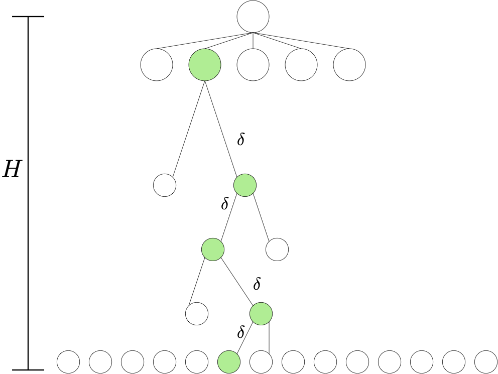
Now, fix $1\le i \le k$ and define $(a_0^*,\dots,a_{H-1}^*)$ by $f(i)=(a_0^*,\dots,a_{H-1}^*)$. Let $s_0^*=s_0$, $s_1^*=(a_0^*)$, $s_2^*=(a_0^*,a_1^*)$, $\dots$, $s_H^*=(a_0^*,\dots,a_{H-1}^*)$. Then, in MDP $M_i$, $r_{a_{H-1}^*}(s_{H-1}^*)=2\delta$ while $r_a(s)=0$ for any other state-action pair.

Note that the optimal reward in $H$ steps from $\perp$ is $2\delta$ and the only policy that achieves this reward is the one that goes through the states in $s_0^*,s_1^*,\dots,s_{H-1}^*$. We can visualize MDP $M_i$ as a tree, as seen on the figure on the right. The green nodes on the figure correspond to the states $s_0^*,s_1^*,\dots,s_{H-1}^*,s_H^*$. Note also that $\mathcal{S}_h = \mathcal{A}^h$ for $0\le h \le H$.

We will now describe the action-value functions of the memoryless policies in $M_i$ as this will be useful later. Fix $0\le h \le H-1$. Then, $q^{\pi}_{H-h}$, by our convention, is defined over $\mathcal{S}_h$. Then, for any $s\in \mathcal{S}_h (=\mathcal{A}^h)$ and $a\in \mathcal{A}$,

\[\begin{align} q^\pi_{H-h}(s,a) = \begin{cases} 2\delta\,, & \text{if } h=H-1, s=s_{H-1}^*, a=a_{H-1}^*\,;\\ v^\pi_{H-h-1}(s_{h+1}^*)\,, & \text{if } h<H-1, s=s_h^*, a=a_h^*\,;\\ 0\,, & \text{otherwise}\,. \end{cases} \label{eq:qpiinfh} \end{align}\]

Note that here $0\le v^\pi_{H-h-1}(g(s,a))\le 2\delta$. We see that for each stage $0\le h \le H-1$, there is only one state-action pair such that the value of $q^\pi_{H-h}$ is nonzero, and in this case the value is in the $[0,2\delta]$ interval.

Now, since the planner induces a policy with suboptimality $\delta$, for the action $A$ it returns it holds that $\mathbb{P}(A\ne a_0^*)\le 1/2$ (any other action than $a_0^*$ incurs zero total expected reward in our construction). Then with $b\ge \log(2H)/\log(2)=\log_2(2H)$ fresh calls, by taking the action $A_0$ that is returned most often in these calls, we get $\mathbb{P}(A_0\ne a_0^*)\le 1/(2H)$. Repeating this process in state $S_1=g(s_0,A_0)$ we get action $A_1$ so that

\[\begin{align*} \mathbb{P}(A_0\ne a_0^* \text{ or } A_1\ne a_1^*) & = \mathbb{P}(A_0\ne a_0^*)+ \mathbb{P}(A_0= a_0^*,A_1\ne a_1^*)\\ & \le \mathbb{P}(A_0\ne a_0^*)+ \mathbb{P}(A_1\ne a_1^*|A_0= a_0^*) \le \frac{1}{2H}+\frac{1}{2H}\,. \end{align*}\]

Now, repeating again the process in state $S_2 = g(S_1,A_1)$ gives $A_2$, etc. Eventually, we get a sequence of actions $A_0,\dots,A_{H-1}$ such that $\mathbb{P}(A_0\ne a_0^* \text{ or } \dots \text{ or } A_{H-1}\ne a_{H-1}^*)\le 1/2$.

By our previous argument (reduction to the “needle” problem), this whole process needs $\Omega(k)$ queries. If the expected number of queries issued by $\mathcal{P}$ is $q$, the expected number of queries issued here is $H \log_2(2H) q$. Hence,

\[q = \Omega\left( \frac{k}{\log_2(2H)H} \right)\,.\]

Let us now consider a choice for $\Phi = (\Phi_h)_{0\le h \le H-1}$ such that $\varepsilon^*(M,\Phi)\le \varepsilon$. For $\Phi_h$ choose first a “JL feature matrix” $\tilde \Phi_h\in \mathbb{R}^{|\mathcal{S}_h| \times d}$ such that Eq. \eqref{eq:featjl} holds. Then let $\Phi_h = \sqrt{2\delta} \tilde \Phi_h$. Choose $\theta_h = v^\pi_{H-h-1}( s_{h+1}^* ) \varphi_h( s_h^*,a_{h}^* )/(2\delta)$ if $h<H-1$ and choose $\theta_h = \varphi_h( s_h^*,a_{h}^* )$, otherwise. Then, by Eq. \eqref{eq:qpiinfh}, for $(s,a)\ne (s_h^*,a_{h}^*)$, $|\varphi_h(s,a)^\top \theta_h-q_{H-h}(s,a)| \le |v^\pi( s_{h+1}^* )| \, |\tilde \varphi_h(s,a)^\top \tilde \varphi_h(s_h^*,a_{h}^*)|\le 2\delta \tau$ and for $(s,a)=(s_h^*,a_{h}^*)$, $\varphi_h(s,a)^\top \theta_h=q_{H-h}(s,a)$. Hence, $\varepsilon^*(M,\Phi)\le \varepsilon$ holds if we set $\tau=\varepsilon/(2\delta)$.

From Eq. \eqref{eq:krange}, $\tilde \Phi_h$ exists if $d\le k$ and

\[\begin{align*} k \le u:=\left\lfloor\exp\left(\frac{d (\frac{\varepsilon}{2\delta})^2}{8}\right)\right\rfloor\,. \end{align*}\]

Recall that $k = \mathrm{A}^H$. Thus, the required claim holds for the case when $\mathrm{A}^H\le u$ (“small horizon case”). In the opposite case (“large horizon”), let $\tilde H$ be the largest positive number such that $\mathrm{A}^{\tilde H}\le u$ holds. Repeating the above argument with horizon $\tilde H$ gives the lower bound $q = \Omega\left( \frac{\mathrm{A}^{\tilde H}}{\log_2(2\tilde H)\tilde H} \right) = \Omega\left( \frac{u}{\log_2(2\tilde H)\tilde H} \right)\,,$ which finishes the proof. $\qquad \blacksquare$

Proof of the JL lemma

For completeness, we include a proof of the JL lemma. The proof uses the so-called probabilistic method The idea of this is that sometimes it is easier to establish the existence of some “good configuration” (like the nearly orthogonal vectors on the unit sphere in the JL lemma) by establishing that such a configuration has positive probability under some probability distribution over possible configurations.

In our case, this works as follows: Let $V_1,\dots,V_k$ be random vectors, each uniformly distributed on the $d$-dimensional unit sphere and so that the distinct vectors in this sequence are pairwise independent of each other. Take $i\ne j$. If we show that $|\langle V_i, V_j \rangle| \le \tau$ holds with probability at least $1-1/k^2$, by a union bound over the $k(k-1)/2$ pairs $1\le i <j \le k$, it follows that $\max_{i\ne j} |\langle V_i,V_j | \le \tau$ holds with probability at least $1/2$, from which, the lemma follows.

Thus, it remains to show that the angle between the random vectors $V_i$ and $V_j$ is “small” with the claimed probability. Since the uniform distribution is rotation invariant and $V_i$ and $V_j$ are independent of each other, $\langle V_i, V_j \rangle$ has the same distribution as $\langle e_1, V_1 \rangle = V_{11}\in [-1,1]$. To see this take a rotation $R$ that rotates $V_i$ to $e_1$; then $\langle V_i, V_j \rangle = \langle R V_i, R^{-1} V_j \rangle = \langle e_1, R^{-1} V_j \rangle$. Now, since $R$ and $V_j$ are independent of each other, $R^{-1} V_j$ is still uniformly distributed on the sphere, hence, $\langle e_1, R^{-1} V_j \rangle$ and $\langle e_1, V_1 \rangle$ share the same distribution.

A tedious calculation shows that for any $x\ge 6$,

\[\begin{align} \mathbb{P}( V_{11}^2 > x/d) \le \exp(-x/4)\,. \label{eq:dgtail} \end{align}\]

(The idea of proving this is to notice that if $X$ is $d$-dimensional standard normal variable then $V=X/\|X\|_2$ is uniformly distributed on the sphere. Then, one proceeds using Chernoff’s method.) The result now follows from \eqref{eq:dgtail} by choosing $x$ so that $\tau^2 = x/d$ holds. $\qquad \blacksquare$

Notes

The lower bound for the discounted case is missing the planning horizon. In the fixed-horizon setting, the lower bound is again missing the horizon when the horizon is large. It remains to be seen whether the extra “horizon terms” in Eq. \eqref{eq:limit} are necessary.
In any case, the main conclusion is that even when we require “strong features”, high-accuracy planning is intractable.
The reader familiar with the TCS literature may recognize a close resemblance to questions studied there which are concerned with the existence of “fully polynomial time approximation schemes” (FPTAS).
There are many open questions. For one, is there a counterpart of the second theorem for the discounted setting?

Bibliographical notes

The idea of using the Johnson-Lindenstrauss lemma in this context is due to Du, Kakade, Wang and Yang (DKWY, for short). The first theorem is a variant of a result from this paper. The second theorem is a variation of Theorem 4.1 from the paper of Du et al. mentioned above who prove the analoge result for global planners. The proof of the lemma also follows the proof given in this paper. The proof of inequality \eqref{eq:dgtail} is given in a paper of Dasgupta and Gupta, which also gives the “full version” of the Johnson-Lindenstrauss lemma which states that logarithmically many dimensions are sufficient to keep pairwise distances between a finite set of points.

Dasgupta, Sanjoy; Gupta, Anupam (2003), “An elementary proof of a theorem of Johnson and Lindenstrauss” link, Random Structures & Algorithms, 22 (1): 60–65

The presentation of the first result which is for “bandits” (fixed horizon problems with $H=1$) follows closely that of a paper by Lattimore, Weisz and yours truly. This, and a paper by van Roy and Dong were both prompted by the DKWY paper, whose initial version focused on the case when $\delta \ll \sqrt{d} \varepsilon$, which made the outlook for designing robust RL methods quite bleak. While it is true that in this high-precision regime nothing much can be done (unless further restricting the features), both papers emphasized that the hardness result disappears when the algorithm can deliver $\delta$ optimal policies with $\delta \gtrsim \sqrt{d} \varepsilon$.