6. online planning - Part II.

PDF Version

In the previous lecture online planning was introduced. The main idea is to amortize the cost of planning by asking a planner to produce an action to be taken at a particular state so that the policy induced by repeatedly calling the planner at the states just visited and then using the action returned by the planner is near-optimal. We have seen that with this, the cost of planning can be made independent of the size of the state space – at least for deterministic MDPs. For this, one can use just a recursive implementation of value iteration, which, for convenience, we wrote using action-value functions and the corresponding Bellman optimality operator, $T$, defined by

(in the previous lecture we used $\tilde T$ to denote this operator, but to reduce clutter from now on, we will drop the tilde).

We have also seen that no procedure can do significantly better in terms of its runtime (or query cost) than this simple recursive procedure. In this lecture we show that these ideas also extend to the stochastic case.

Sampling May Save the Day?

Assume now that the MDP is stochastic. Recall the pseudocode of the recursive form of value iteration from the last lecture that computes $(T^k \boldsymbol{0})(s,\cdot)$:

1. define q(k,s):
2.  if k = 0 return [0 for a in A] # base case
3.  return [ r(s,a) + gamma * sum( [P(s,a,s') * max(q(k-1,s')) for s' in S] ) for a in A ]
4. end

Obviously, the size of the state space creeps in because in line 3 we need to calculate an expected value over the next state distribution at $(s,a)$. As noted beforehand, in deterministic systems when a simulator is available, the sum over the next-states can be replaced with a single simulator call. But the reader may remember from Probability 101 that sampling allows one to approximate expected values, where the error of approximation is independent of the cardinality of the set over which we average the values. Here, this set is $\mathcal{S}$, the state space. This is extremely lucky!

To quantify the size of these errors, we recall Hoeffding’s inequality:

Lemma (Hoeffding’s Inequality): Given $m$ independent, identically distributed (i.i.d.) random variables that take values in the $[0,1]$ interval, for any \(0 \leq \zeta < 1\), with probability at least \(1 - \zeta\) it holds that

Letting $S_1’,\dots,S_m’ \stackrel{\textrm{i.i.d.}}{\sim} P_a(s)$ for some state-action pair $(s,a)$ and $v:S \to [0,v_{\max}]$, by this result, for any $0\le \zeta <1$, with probability $1-\zeta$,

This suggests the following approach: For each state action pair $(s,a)$ draw $S_1’,\dots,S_m’ \stackrel{\textrm{i.i.d.}}{\sim} P_a(s)$ and store it in a list $C(s,a)$. Then, whenever for some function $v$ we need the value of $\langle P_a(s), v \rangle$, just use the sample average

Plugging this approximation into our previous pseudocode gives the following new code:

1. define q(k,s):
2.  if k = 0 return [0 for a in A] # base case
3.  return [ r(s,a) + gamma/m * sum( [max(q(k-1,s')) for s' in C(s,a)] ) for a in A ]
4. end

The total runtime of this function is now $O( (m\mathrm{A})^{k+1} )$. What is important is that this will give us a compute time independent of the size of the state space as long as we can show that $m$ can be set independently of $\mathrm{S}$ while meeting our target for the suboptimality of the induced policy.

This pseudocode sweeps under the rug on who creates the lists $C(s,a)$ and when? A simple and effective approach is to use “lazy evaluation” (or memoization): Create $C(s,a)$ at the first time it is needed (and do not create it otherwise). An alternative to the approach we follow here is to avoid storing these lists and just create them on demand. Both procedures are valid, but we will stick to the procedure that creates the lists only once and will comment on the other approach at the end in the notes.

Good Action-Value Approximations Suffice

As a first step towards understanding the strength and weaknesses of this approach, let us define $\hat T: \mathbb{R}^{\mathcal{S}\times\mathcal{A}} \to \mathbb{R}^{\mathcal{S}\times\mathcal{A}}$ by

With the help of this definition, when called with state $s=s_0$, the planner computes

The conciseness of this formulae, if anything, must please everyone!

Let us now turn to the question of whether the policy $\hat \pi$ induced by this planners is a good one. We start with a lemma that parallels our earlier result that bounded the suboptimality of a policy that is greedy w.r.t. a function over the states as a function of how well the function approximates the optimal value function. To state the lemma, we need the analog of optimal value functions but with action values.

Suboptimality of $\epsilon$-optimizing policies

Define

We call this function $q^*$ the optimal action-value function (in our MDP). The function \(q^*\) is easily seen to satisfy \(M q^* = v^*\) and thus also \(q^* = T q^*\). The promised lemma is as follows:

Lemma (Policy error bound - I.): Let $\pi$ be a memoryless policy and choose a function $q:\mathcal{S}\times\mathcal{A} \to \mathbb{R}$ and $\epsilon\ge 0$. Then, the following hold:

1. If $\pi$ is $\epsilon$-optimizing in the sense that \(\sum_a \pi(a\vert s) q^*(s,a) \ge v^*(s)-\epsilon\) holds for every state $s\in \mathcal{S}$ then $\pi$ is $\epsilon/(1-\gamma)$ suboptimal: \(v^\pi \ge v^* - \frac{\epsilon}{1-\gamma} \boldsymbol{1}\,.\)

2. If $\pi$ is greedy with respect to $q$ then $\pi$ is $2\epsilon$-optimizing with \(\epsilon= \|q-q^*\|_\infty\) and thus

For the proof, which is partially left to the reader, we need to introduce a bit more notation. In particular, for a memoryless policy, define the operator $M_\pi: \mathbb{R}^{\mathcal{S}\times \mathcal{A}} \to \mathbb{R}^{\mathcal{S}}$:

With the help of this operator the condition that $\pi$ is greedy with respect to $q$ can be written as

Further, the second claim of the lemma can be stated in the more concise form $M_\pi q^* \ge v^* - 2\epsilon\boldsymbol{1}$.

For future reference, we will also find it useful to define $P_\pi: \mathbb{R}^{\mathcal{S}\times \mathcal{A}} \to \mathbb{R}^{\mathcal{S}\times \mathcal{A}}$:

Note that here we abused notation as $P_\pi$ has already been used to denote the operator that maps functions of the states to functions of the state. From the context, the meaning of $P_\pi$ will always be clear.

Proof: The first part of the proof is standard and is left to the reader. For the second part note that

Then use the first part. \(\qquad \blacksquare\)

Suboptimality of almost $\epsilon$-optimizing policies

There are two issues that need to be taken care of. One is that the planner is randomizing when computing the values $Q_H(s_0,\cdot)$. What happens when the random next states obtained from the simulator are not “representative”? We cannot expect the outcome of this randomized computation to be precise! Indeed, the best we can expect is that the outcome is “accurate” with some probability, hopefully close to one. In fact, from Hoeffding’s inequality, we see that if we want to achieve small errors in the computation for some target probability, we need to increase the sample size. But Hoeffding’s inequality, in all cases, allows errors which are uncontrolled on some failure event.

All in all, the best we can hope for is that with each call, $Q_H(s_0,\cdot)$ is a good approximation to \(q^*(s_0,\cdot)\) outside of some “failure event” $\mathcal{F}$ whose probability we will control separately. Let us say the probability of $\mathcal{F}$ is at most $\zeta$:

Here, $\mathbb{P}_{s_0}$ denotes the probability measure induced by the interaction of the planner and the MDP simulator on an appropriate probability space. We will choose $\mathcal{F}$ so that on $\mathcal{F}^c$, the complementer of $\mathcal{F}$ (a “good” event), it holds that

Then, on $\mathcal{F}^c$,

That is, on the good event $\mathcal{F}^c$, the action $A$ returned by the planner is $2\epsilon$ optimizing at state $s_0$.

Let $\hat \pi(a \vert s_0)$ denote the probability that action $A$ returned by the planner is $a$: \(\hat \pi(a \vert s_0)=\mathbb{P}_{s_0}(A=a)\). Then,

In words, with probability at least $1-\zeta$, $\hat \pi$ chooses $2\epsilon$-optimizing actions: The policy is almost $2\epsilon$-optimizing. While this is not as good as always choosing $2\epsilon$-optimizing actions, we expect that as $\zeta\to 0$ the difference in performance between $\hat \pi$ and a policy that always chooses $2\epsilon$-optimizing actions disappears because performance is expected to depend on action probabilities in a continuous fashion. The next lemma makes this precise:

Lemma (Policy error bound II): Let $\zeta\in [0,1]$, $\pi$ be a memoryless policy that selects $\epsilon$-optimizing actions with probability at least $1-\zeta$ in each state. Then,

Proof: By Part 1 of the previous lemma, it suffices to show that $\pi$ is \(\epsilon+2\zeta \|q^*\|_\infty\)-optimizing in every state. This follows from algebra and is left to the reader. \(\qquad \blacksquare\)

Error control

What remains is to show that with high probability, the error $\delta_H$, defined in \(\eqref{eq:d0def}\) is small. Intuitively, $\hat T \approx T$. To firm up this intuition, we may note that for any fixed $q\in \mathbb{R}^{\mathcal{S}\times \mathcal{A}}$ function over the state-action pairs such that \(\|q\|_\infty \le \frac{1}{1-\gamma}\) and for any fixed $(s,a)\in \mathcal{S}\times \mathcal{A}$, by Eq. \(\eqref{eq:hoeffbop}\) and the choice of the sets $\mathcal{C}(s,a)$, with probability $1-\zeta$,

where, for brevity, we introduced $v = Mq$ in the above formula.

Union bounds

So we know that for any fixed state-action pair $(s,a)$, outside of a low probability event, $(\hat T q)(s,a)$ is close to $( T q)(s,a)$. But can we conclude from this that, outside of some low probability event, $(\hat T q)(s,a)$ is close to $( T q)(s,a)$ everywhere?

To answer this question, it will be easier to turn it around and just try to come up with some event that, on the one hand, has low probability, while, in the other hand, outside of this event, $(\hat T q)(s,a)$ is close to $( T q)(s,a)$ regardless of $(s,a)$.

Denoting by $\mathcal{E}(s,a)$ the event when $(\hat T q)(s,a)$ is not close to $( T q)(s,a)$, i.e.,

it is clear that if $\mathcal{E} = \cup_{(s,a)} \mathcal{E}(s,a)$ then outside of $\mathcal{E}$, none of $\mathcal{E}(s,a)$ holds and hence

But how large can the probability of $\mathcal{E}$ be? For this, recall the following elementary result, which follows directly from the properties of measures:

Lemma (Union Bound): For any probability measure $\mathbb{P}$ and any countable sequence of events \(A_1, A_2, \ldots\) of the underlying measurable space,

By this result, using that $\mathcal{S}\times \mathcal{A}$ is finite,

If we want this probability to be $0\le \zeta’\le 1$, we can set $\zeta = \frac{\zeta’}{\mathrm{S}\mathrm{A}}$ and conclude that with probability $1-\zeta’$, for any state-action pair $(s,a)\in \mathcal{S}\times \mathcal{A}$,

The following diagram summarizes the idea of union bounds:

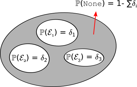
To control the error of some bad event happening, we can break the the bad event into a number of elementary parts. By controlling the probability of each such part, we can control the probability of the bad event, or, alternatively, control the probability of the complementary “good” event. The worst case for controlling the probability of the bad event is if the elementary parts do not overlap, but the argument of course works even in this case.

Returning to our calculations, from the last formula we see that the errors grew a little compared to \(\eqref{eq:basicerror}\), but the growth is modest: the errors scale with the logarithm of the number of state-action pairs. While this logarithmic error-growth is mild, it is unfortunate that the number of states appears here. To control the errors, by this formulae we would need to choose $m$ to be proportional to the logarithm of the size of the state space, which is better than a linear dependence, but still. One must wonder whether this dependence is truly necessary? If it was, there would be a big gap between the complexity of planning in deterministic and stochastic MDPs. We should not give in for this just yet!

Avoiding dependence on state space cardinality

The key to avoiding the dependence on the cardinality of the state is to avoid taking union bounds over the whole state-action set. That this may be possible follows from that, thinking back to the recursive implementation of the planner, we can notice that the planner does not necessarily rely on all the sets $\mathcal{C}(s,a)$.

To get a handle on this, it will be useful to introduce a notion of a distance induced by the set $\mathcal{C}(s):=\cup_{a\in \mathcal{A}}\mathcal{C}(s,a)$ between the states. This distance between states $s$ and $s’$ (denoted by $\text{dist}(s,s’)$) will be the smallest number of steps that we can take to get from $s$ to $s’$, if in each step we choose one “neighbouring” state to the last state, starting from state $s$. Formally, this is the length $n$ of the shortest sequence $s_0,s_1,\dots,s_n$ such that $s_0=s$, $s_n = s’$ and for each $i\in [n]$, $s_i \in \mathcal{C}(s_{i-1})$ (this is the distance between states in the directed graph over the states with edges induced by $\mathcal{C}$).

With this, for $h\ge 0$, define

as the set of states accessible from $s_0$ by at most $h$ steps. Note that this is a nested sequence of sets and $\mathcal{S}_0 = {s_0}$, $\mathcal{S}_1$ contains $s_0$ and its immediate “neighbors”, etc.

We may now observe that in the calculation of $Q_H(s_0,\cdot)$ when function $q$ is called with a certain value of $0\le k \le H$, for the state that appears in the call we have

This can be proved by induction on $k$, starting with $k=H$.

Taking into account that when $q$ is called with $k=0$, the sets $\mathcal{C}(s,a)$ are not used (line 2), we see that only states $s$ from $\mathcal{S}_{H-1}$ are such that the calculation ever uses the set $\mathcal{C}(s,a)$. Since $|\mathcal{C}(s,a)|=m$,

and in particular, $\mathcal{S}_{H-1}\le (mA)^H$, which is independent of the size of the state space. Of course, all along, we knew this very well: This is why the total runtime is also independent of the size of the state space.

The plan is to take advantage of this to avoid a union bound over all possible state-action pairs. We start with a recursive expression for the errors.

Recall that \(\delta_H = \| (\hat T^H \boldsymbol{0})(s_0,\cdot)-q^*(s_0,\cdot)\|_\infty\). By the triangle inequality,

Now, observing that

we see that

In particular, defining

we see that

where we use the notation \(\| q \|_{\mathcal{U}} = \max_{s\in \mathcal{U},\max_{a\in \mathcal{A}}} |q(s,a)|\). More generally, we can prove by induction on $1\le h \le H$ (starting with $h=H$) that

while

where the last inequality uses that $r_a(s)\in [0,1]$, which we shall assume for simplicity. Unfolding this recursion for $(\delta_h)_h$, letting

we get

We see that the first term in the sum on the right-hand side (in the parenthesis) is controlled by $H$. It remains to show that $\varepsilon’$ can also be controlled (by choosing $m$ appropriately).

In fact, notice that $\varepsilon’ / (1 - \gamma)$ is the maximum-norm error with which \(\hat T q^*\) approximates \(q^* = T q^*\), but only for states in \(\mathcal{S}_{H-1}\) we need to control this error. By our earlier argument, this set has at most \((mA)^H\) states, hence, it is believable that this error can be controlled even when $m$ is chosen independently of the number of states.

Controlling \(\| \hat T q^* - q^* \|_{\mathcal{S}_{H-1}}\)

Since \(\mathcal{S}_{H-1}\) has only $(mA)^H$ states in it, one’s first instinct is to take a union bound over the error events for the states in this set. The trouble is that the set \(\mathcal{S}_{H-1}\) itself is random. As such, it is not clear, what the failure events should be? And how many failure events are we going to have? The size of this set is also random! Notice that if \((A_i)_{i\in [n]}\) are some events with \(\mathbb{P}(A_i)\le \delta\) and \(I_1,\dots,I_k\in [n]\) are random indices, it does not hold that \(\mathbb{P}( \cup_{j=1}^k A_{I_j}) \le k \delta\): One cannot apply the union bound to randomly chosen events. In fact, in the worst case, \(\mathbb{P}( \cup_{j=1}^k A_{I_j}) = n \delta\).

To exploit that \(\mathcal{S}_{H-1}\) is a small set, we need to use one more time the structure. The reason that the randomness of \(\mathcal{S}_{H-1}\) is not going to matter too much is because of the special way this set is constructed. First of all, clearly, \(s_0\in \mathcal{S}_{H-1}\) always and at this state the error \(\|(\hat T q^*)(s_0,\cdot)- Tq^*(s_0,\cdot)\|_\infty\) is under control by Hoeffding’s inequality. Next, we may consider the neighbors of \(s_0\). If \(S\in \mathcal{C}(s_0)\), either \(S=s_0\), in which case we already know that the error at \(S\) is under control, or \(S\) is a “bona fide neighbor” and we can think of then generating the elements in \(\mathcal{C}(S,a)\) just inside the call of $q$. Ultimately, the error at such a neighbor is under control because, by definition, all the sets \(\mathcal{C}(s,a)\) (with $(s,a)$ sweeping through all possible state-action pairs) are independently chosen.

This suggests that we should consider the chronological order in which in the recursive call of function $q$ the states in \(\mathcal{S}_{H-1}\) appear. Let this order be $S_1,S_2,\dots,S_n$, where $n = 1+(mA)+\dots+(mA)^{H-1}$, $S_1=s_0$, $S_2$ is the second state that $q$ is called on (necessarily, \(S_2\in \mathcal{C}(s_0)\)), \(S_3\) is the third such state. Note that states may reappear in this sequence multiple times. Furthermore, by construction, \(\mathcal{S}_{H-1} = \{ S_1,\dots,S_n \}\). Also note that the length of this sequence is not random: This length is exactly the number of times $q$ is called, which is clearly not random.

That \(\| \hat T q^* - q^* \|_{\mathcal{S}_{H-1}}=\| \hat T q^* - Tq^* \|_{\mathcal{S}_{H-1}}\) is under control directly follows from the next lemma:

Lemma: Assume that the immediate rewards belong to the $[0,1]$ interval. For any $0\le \zeta \le 1$ with probability $1-\mathrm{A}n\zeta$, for any $1\le i \le n$,

where \(\Delta\) is given by \(\eqref{eq:basicerror}\).

Proof: Recall that $\mathcal{C}(s,a) = (S_1’(s,a),\dots,S_m’(s,a))$ where (i) the \((\mathcal{C}(s,a))_{(s,a)}\) are mutually independent and (ii) for any $(s,a)$, $(S_i’(s,a))_i$ is an i.i.d. sequence with common distribution $P_a(s)$.

For \(s\in \mathcal{S}\), \(a\in \mathcal{A}\), \(C\in \mathcal{S}^m\), let

(as earlier, $s’\in C$ means that $s’$ is an element of the set composed of the elements in the sequence $C$). Recall that by the definition of $\hat T$ and the properties of $q^*$,

Fix \(1 \le i \le n\). Let \(\tau = \min\{ 1\le j \le i\,:\, S_j = S_i \}\). That is, $\tau$ is the time when $S_i$ first appears in the sequence \(\{S_i\}_i\).

Fix $a\in \mathcal{A}$. We claim that given \(S_{\tau}\), \((S_j'(S_{\tau},a))_{j=1}^m\) is i.i.d. with common distribution \(P_a(S_{\tau})\). That is, for any \(s,s_1',\dots,s_m'\in \mathcal{S}\),

Note that given this, for any $\Delta\ge 0$, by \(\eqref{eq:dub}\),

for some binary valued functions $\phi_1$, $\dots$, $\phi_i$ where for $1\le j \le i$, $\phi_j$ is defined so that

holds if and only if $S_j=s, S_{1:j-1}=s_{1:j-1}$ holds, where $s\in \mathcal{S}$ and $s_{1:j-1}\in \mathcal{S}^{j-1}$ are arbitrary so that $s\not\in s_{1:j-1}$. That such functions exist follows because for any sequence $s_{1:j}$ to verify whether $S_{1:j}=s_{1:j}$ the knowledge of the sets $\mathcal{C}(s_1),\dots,\mathcal{C}(s_{j-1})$ suffices: The appropriate function should first check $S_1=s_1$, then move on to checking $S_2=s_2$ only if $S_1=s_1$ holds, etc.

Now, notice that by our assumptions, for $s\not\in s_{1:j-1}$, $\mathcal{C}(s,a)$ and $\phi_j( s,s_{1:j-1},\mathcal{C}(s_1),\dots,\mathcal{C}(s_{j-1}) )=1$ are independent of each other. Hence,

Plugging this back into the previous displayed equation, “unrolling” the expansion done using the law of total probability, we find that

Now, choose $\Delta = \Delta(\zeta,m)$ from \(\eqref{eq:basicerror}\) so that, thanks to $|q^*|_\infty \le 1/(1-\gamma)$, for any fixed $(s,a)$, \(\mathbb{P}( g(s,a,\mathcal{C}(s,a)) > \Delta(\zeta,m) )\le \zeta\) Plugging this in into the previous display we get

The claim the follows by a union bound over all actions and all $1\le i \le n$. \(\qquad \blacksquare\)

Final error bound

Putting everything together, we get that for any $0\le \zeta \le 1$, the policy $\hat \pi$ induced by the planner is $\epsilon(m,H,\zeta)$-optimal with

Thus, to obtain a planner that induces a $\delta$-optimal policy, we can set $H$, $\zeta$ and $m$ so that each term above contributes at most $\delta/3$:

For $H$ we get that we can set $H = \lceil H_{\gamma,(1-\gamma)\delta/6}\rceil$. We can also set $\zeta = (1-\gamma)^2\delta/6$. To solve for the smallest $m$ that satisfies the last inequality, recall that $n = (mA)^H$. To find the critical value of $m$ note the following elementary result which we cite without a proof:

Proposition: Let $a>0$, $b\in \mathbb{R}$. Let \(t^*=\frac{2}{a}\left[ \log\left(\frac1a\right)-b \right]\). Then, for any positive real $t$ such that $t\ge t^*$,

From this, defining

and

if $m \ge m^*$ then all the inequalities are satisfied. Putting things together, we thus get the following result:

Theorem: Assume that the immediate rewards belong to the $[0,1]$ interval. There is an online planner such that for any $\delta\ge 0$, in any discounted MDP with discount factor $\gamma$, the planner induces a $\delta$-optimal policy and uses at most \(O( (m^* \mathrm{A})^H )\) elementary arithmetic and logic operations per its calls, where $m^*(\delta,\mathrm{A})$ is given by \(\eqref{eq:mstar}\) and $H = \lceil H_{\gamma,(1-\gamma)\delta/3}\rceil$.

Overall, we see that the runtime did increase compared to the deterministic case (apart from logarithmic factors, in the above result $m = H^7/\delta^2$ whereas in the deterministic case $m=1$!), but we managed to get a runtime that is independent of the cardinality of the state space. Again, what is troubling is the exponential dependence on the effective horizon, though as we have seen, in the worst-case, this is unavoidable. In the next lectures we will consider proving the planner with extra information so that this exponential dependence can be avoided.

Notes

Sparse lookahead trees

The idea of the algorithm that we analyzed comes from a paper by Kearns, Mansour and Ng from 2002. In their paper they consider the version of the algorithm which creates a fresh “new” random set $\mathcal{C}(s,a)$ in every recursive call. This makes it harder to see their algorithm as approximating the Bellman operator, but in effect, the two approaches are by and large the same. In fact, if we introduce $H$ random operators, $\hat T_1$, $\dots$, $\hat T_H$ which are the same as $\hat T$ above but $\hat T_h$ has its own “private” sets $( \hat C_h(s,a) )_{(s,a)}$, then their algorithm can be written as computing

It is not hard to modify the analysis given here to accommodate this change. With this, one can also interpret the calculations done by the algorithm as backing up values in a “sparse lookahead tree” built recursively from $s_0$.

Much work has been devoted to improving these basic ideas and eventually these ideas led to various Monte-Carlo tree search algorithms, including yours truly’s UCT. In general, these algorithms attempt to improve on the runtime by building the trees when they need to be built. As it turns out, a useful strategy here is to expand nodes which in a way hold the greatest promise to improve the value at the “root”. This is known as the “optimisism in planning”. Note that A* (and its MDP relative, AO) are also based on optimism: A’s admissible heuristic functions in our language correspond to functions that upper bound the optimal value. The definite source on MCTS theory as of today is Remi Munos’s monograph.

Measure concentration

Hoeffding’s inequality is a special case of what is known as measure concentration. This phrase refers to that the empirical measure induced by a sample is a good approximation to the whole measure. The simplest case is when one just compares the means of the measures (the empirical and the sample-generating one), giving rise to concentration inequalities around the mean. Hoeffding’s inequality is an example. What we like about Hoeffding’s inequality (besides that it is simple) is that the failure probability, $\delta$ (later $\zeta$) appears inside a logarithm. That means, that the price of being more stringent is mild. When the exact dependence is of type that appears in Hoeffding’s inequality (i.e., $\sqrt{ \log(1/\delta)})$), we say that the deviation of the subgaussian type because Gaussian random variables also satisfy an inequality like this. Concentration of measure and concentration inequalities are a central topic in probability theory, with separate books devoted to them. A few favourites are given at the end of this notes . For learning purposes, Pollard’s mini-book is nice (but all these books have pros and cons), or Vershynin’s book.

The comparison inequality

The comparison inequality between the logarithm and the linear function is given as Proposition 4 here. The proof is based on two observations: First, it is enough to consider the case when $b=0$. Then, if $a\ge 1$, the result is trivial, while for $a< 1$, the guess is based on doubling the value where the growth rate of $t\mapsto at$ matches that of $t\mapsto \log(t)$.

A model-centered view and random operators

A key idea of this lecture is that $\hat T$ is a good (random) approximation to $T$, hence, it can be used in place of $T$. One can also tell this story by saying that the data underlying $\hat T$ gives a random approximation to the MDP; the transition probabilities of this random approximating MDP would be defined using

It may seem quite miraculous that with only a few elements in $C(s,a)$ (i.e., small $m$) we get a good approximation to the next state distribution. But so is the magic of randomness! Using a random operator (or a sequence of them, if, as outlined above, one uses a fresh set of random next state every time an update is calculated) in a dynamic programming method has been coined empirical dynamic programming by Haskell et al..

A bigger point is that for a model to be a “good” approximation to the “true MDP”, it suffices that the Bellman optimality operator that it induces is a “close” approximation to the Bellman optimality operator of the true MDP.

This in fact brings us to our next topic, which is what happens when the simulator is imperfect?

Imperfect simulation model?

We can rarely expect simulators to be perfect. Luckily, not all is lost in this case. As noted above, if the simulator induced an MDP whose Bellman optimality operator is in a way close to the Bellman optimality operator of the true MDP, we expect the outcome of planning to be still a good policy in the true MDP.

In fact, the above proof has already all the key elements in place to show this. In particular, it is not hard to show that if $\hat T$ is a $\gamma$ max-norm contraction and $\hat q^*$ is its fixed point then

which, combined with the our first lemma of this lecture on the policy error bound gives that the policy that is greedy with respect to $\hat q^*$ is

optimal in the MDP underlying $T$. We will return to this in later lectures. In particular, in batch reinforcement learning, one of the basic methods is to learn a “model” of the environment and as such it is inevitable to study the error that results from modelling errors. See Lecture 17 and Lecture 18.

Monte-Carlo methods

We saw in homework 0 that randomization may help a little, and today we saw that it can help in a more significant way. A major lesson again is that representations do matter: If the MDP is not given with a “generative simulator”, getting such a simulator may be really hard. This is good to remember when it comes to learning models:

One should insist on learning models that make the job of planners easier.

Generative models are one such case, provably, as we have seen in today’s lecture put together with our previous lower bound that involved the number of states. Randomization, more generally, is a powerful tool in computing science, which brings us to a somewhat philosophical question: What is randomness? Does “true randomness” exist? Can we really build computers to harness this?

True randomness?

What is the meaning of “true” randomness? The margin is definitely not big enough to explain this. Hence, we just leave this there, hanging, for everyone to ponder about. But let’s also note that this is a thoroughly studied question in theoretical computing science, with many beautiful results and even books. Arora and Barak’s book on computational complexity (Chapters 7, 20 and 21) is a good start for exploring this.

Can we recycle the sets $C(s,a)$ between the calls?

If simulation is expensive, it may be tempting to recycle the sets between calls of the planner. After all, even if we recycle these sets, \(\hat{\pi}\) will have the property that it selects $\epsilon$-optimizing actions with high probability at every state. However, this may not be a good idea. The reader is challenged to think about what can go wrong? The proof actually uses that the planner construct a new random operator $\hat T$ with every call. But where is this used?

The ubiquity of continuity arguments in the MDP literature

All the computations that we do with MDPs tend to be approximate. We evaluate policies approximately. We compute a Bellman back approximately. We have approximate models. We greedify approximately. If any of these operations could enlarge small errors, none of the approximate methods would work. The study of approximate computations (which is a necessity if one faces large MDPs) is a study of the sensitivity of the values of the resulting policies to the errors introduced in the computations. This, in numerical analysis, would be called error analysis. In other areas of mathematics, this is called sensitivity analysis. In fact, sensitivity analysis often involves computing derivatives to see how fast outputs change as the inputs change (which is that data that will be approximated). What should we be taking derivatives with respect to here? Well, it is always the data that is being changed. One can in fact use differentiation based sensitivity analysis everywhere. This has been tried a little in the “older” MDP literature and is also related to policy gradient theorems (that we will learn about laters). However, perhaps there are more nice things to be discovered about this approach.

From local to online access

The algorithm that is analyzed in this lecture requires local access simulators. This is better than requiring global access, but worse than requiring online access. It remains an open question of whether with online access, one can also get a similar result than shown in the present lecture and if not, whether the sample complexity of planning remains finite under this setting.

When the state space is small

For finite state-action MDPs where the rewards and transition probabilities are represented using tables, a previous lecture’s main result established that an optimal policy of the MDP can be calculated by using at most $O(H\textrm{poly}(S,A))$ arithmetic and logic operations ($H=1/(1-\gamma)$ here). In the current lecture we saw that even when $S$ is unbounded, given a simulator with local access, $\tilde{O}((AH^7/\delta^2)^H)$ such elementary operations and calls to a simulator are sufficient. In a finite MDP, depending on the values of $S,A$ and $H$, either policy iteration, or the online planner that builds the tree will be faster. But policy iteration (and value iteration) as described previously used a table representation. The question then arises of what is the sample complexity of planning with a simulator access to a finite MDP? If planning means outputting a policy, the complexity needs to scale with $S$. In the presence of global access simulators, a simple approach, is to sample an appropriate number of next states for each state-action pair to build an empirical (but “sparse”) transition model and use this in connection with any MDP solver. We will see later in Lecture 18 that in this case $O(H^3 SA/\delta^2)$ samples (or $H^3/\delta^2$ samples per state-action pair) are sufficient to obtain a $\delta$-optimal policy.

In the case of online planning with global access, the sample complexity cannot be worse, but it is unclear whether it can be improved. Similarly, it is unclear what the complexity is in the case of either local or online access.

References

• Kearns, M., Mansour, Y., & Ng, A. Y. (2002). A sparse sampling algorithm for near-optimal planning in large Markov decision processes. Machine learning, 49(2), 193-208. [link]
• David Pollard (2015). A few good inequalities. Chapter 2 of a book under preparation with working title “MiniEmpirical”. [link]
• Stephane Boucheron, Gabor Lugosi and Pascal Massart (2012). Concentration inequalities: A nonasymptotic theory of indepndence. Clarendon Press – Oxford. [link]
• Roman Vershynin (2018). High-Dimensional Probability: An Introduction with Applications in Data Science. [link]
• M. J. Wainwright (2019) High-dimensional statistics: A non-asymptotic viewpoint. Cambridge University Press.
• Lafferty J., Liu H., & Wasserman L. (2010). Concentration of Measure. [link]
• Lattimore, T., & Szepesvári, C. (2020). Bandit algorithms. Cambridge University Press.
• William B. Haskell, Rahul Jain, and Dileep Kalathil. Empirical dynamic programming. Mathematics of Operations Research, 2016.
• Sanjeev Arora and Boaz Barak (2009). Computational Complexity: A Modern Approach. Cambridge University Press.
• Remi Munos (2014). From Bandits to Monte-Carlo Tree Search: The Optimistic Principle Applied to Optimization and Planning. Foundations and Trends in Machine Learning: Vol. 7: No. 1, pp 1-129.